Achievement
Featured

Launched Logik v1
Successfully launched the first major release of Logik, an educational computational logic framework built in Java. It allows users to build and simulate complex logic circuits.
Successfully launched the first major release of Logik, an educational computational logic framework built in Java. It allows users to build and simulate complex logic circuits.
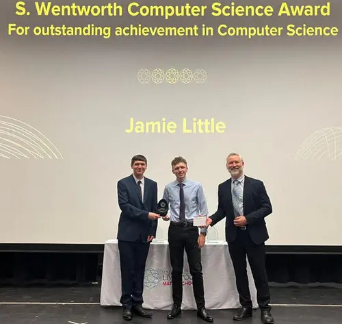
Presented the Computer Science Award at the University of Liverpool Maths School Awards Evening 2025, in recognition of outstanding achievement in Computer Science.
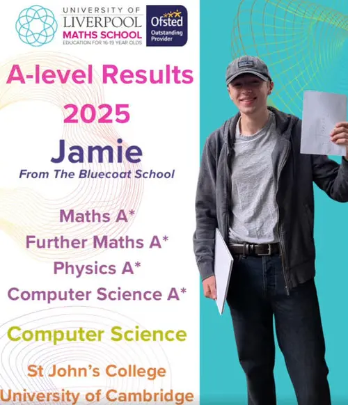
A* in Maths, Further Maths, Physics, and Computer Science. Heading to St John's College, University of Cambridge to read Computer Science.
A from-scratch Raft consensus library in Rust, paired with a fault-tolerant key–value store over gRPC.
A working implementation of the Raft consensus algorithm, built from scratch in Rust. The core Raft protocol — leader election, log replication, and safety — runs inside a single-threaded async event loop and sits underneath a replicated key–value store accessible over gRPC.
Raft is a protocol for getting a group of machines to agree on a sequence of commands, even when some of them crash or lose connectivity. All three subproblems are tackled separately:
On top of Raft sits a concurrent key–value store backed by a DashMap. Clients call Put, Get, and Delete via gRPC. Reads are served locally from whichever replica you hit; writes go through the leader and are replicated before being acknowledged.
Every log entry is written to a JSON-line file (the write-ahead log) before a client gets a response. On restart the log is replayed to restore state. When the log grows large, the node takes a snapshot of the state machine and discards older entries.
The same Raft core can run in two modes:
.proto definition.tokio channels with zero network overhead. The integration tests use this to exercise the full consensus protocol deterministically, without races or real latency.# In-memory demo — no networking needed
cargo run --bin demoThe demo starts a 3-node cluster, runs a leader election, replicates three key–value pairs, and shows that every replica ends up with the same data.
For a real gRPC cluster, see the README.
See the Raft Consensus notes for the theory behind the algorithm.
A professional-grade digital logic circuit simulator with real-time event-driven execution and custom IC packaging.
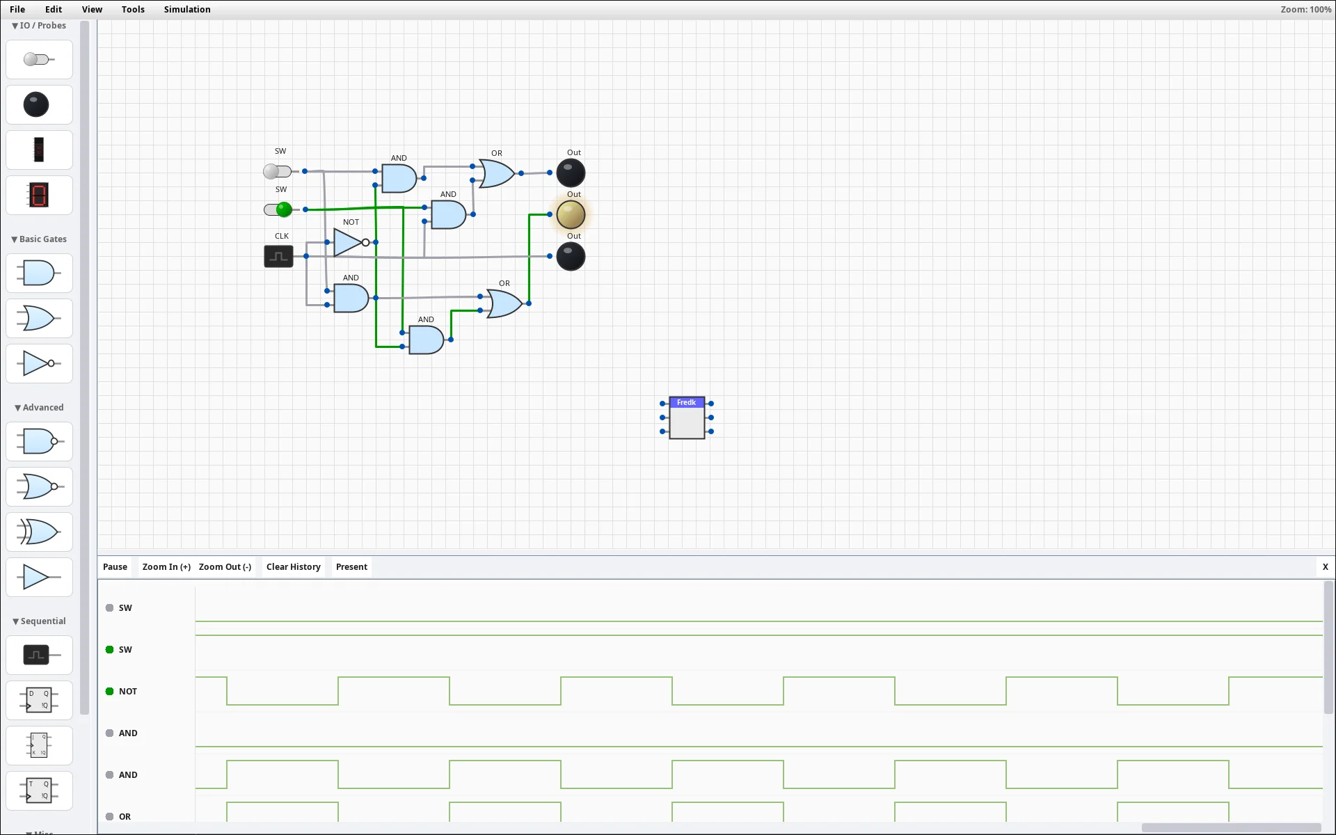
LogiK is a cross-platform digital logic simulator designed for students and engineers. Unlike basic simulators, LogiK focuses on the intersection of visual design and rigorous systems engineering, providing features like gate propagation delay simulation and custom “Black Box” integrated circuit (IC) packaging.
Built using Java 17 and JavaFX, the project leverages a highly decoupled architecture. The simulation core is separated from the rendering layer, ensuring that even large-scale circuits remain responsive.
LogiK makes computer architecture tangible. It bridges the gap between discrete mathematics and physical hardware implementation.
R for rotation, Ctrl+L for auto-layout, and Space to toggle simulation state.You can download the portable JAR and run it locally on any system with Java 17+.
Download LogiK v1.3.1 (Portable JAR)
Latest version: v1.3.1 (Released January 2026)
A fully featured, browser-based raytracer built from scratch in TypeScript with a live XML scene editor.
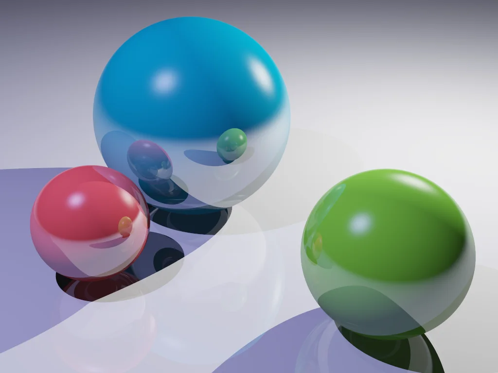
This project is a custom-built rendering engine that draws pixel-by-pixel to an HTML Canvas, implementing core raytracing mathematics from first principles. It features an integrated live editor allowing you to configure scenes using custom XML markup with real-time visual updates.
For every pixel on the canvas, the engine:
kS and shininess exponent alphaS<scene>
<ambient-light colour="#050505"/>
<point-light x="-2" y="2" z="1" colour="#FFFFFF" intensity="80"/>
<point-light x="2" y="-2" z="1" colour="#AAAAFF" intensity="60"/>
<plane
x="0" y="-1" z="5"
nx="0" ny="1" nz="-0.2"
colour="#222222" reflectivity="0.6"
/>
<bumpy-sphere
x="0" y="0" z="3.5" radius="0.7"
colour="#FFFFFF" kS="0.8" alphaS="20"
bump-map="metal.png" bump-scale="15"
/>
</scene>Built with TypeScript, Vite, and the HTML Canvas API. The rendering loop processes pixels in batches to avoid blocking the UI thread. The engine is entirely client-side — no server, no WebGL, just raw pixel manipulation on a <canvas>. The live editor uses CodeMirror 6 for syntax highlighting and real-time parsing of the custom XML scene format.
The Web Raytracer makes the rendering equation tangible. It bridges the gap between the mathematical models covered in the Graphics course and their concrete implementation in code.
See the Computer Graphics revision notes for the underlying theory on ray tracing, shading models, and rendering techniques.
Mathematics, Further Mathematics, Physics, Computer Science.
Orchestrated and delivered Computer Science workshops for Year 12 students. Covered practical programming techniques, foundational algorithmic concepts, and introductory game theory (including the Prisoner's Dilemma).
Course notes, revision guides, and technical writing
Get new notes by email
No spam, just a notification when I publish something new.
14 modules with in-depth revision notes, grouped by Part, term, and paper.
A few days ago, I heard a rumour that Claude had solved the Navier–Stokes problem. My reaction was fairly simple: I will believe it when I see it.
Apparently OpenAI heard a version of the same rumour.
On 1 September, after hearing that two Millennium Prize problems might have been resolved, OpenAI began testing a new internal model against all of the remaining open Millennium problems and several other research questions. On 8 September, it published what it says is a solution to Navier–Stokes, together with an analytical proof and a complete formalisation in Lean.
That last part matters. There is an enormous difference between an AI producing a hundred pages of convincing-looking mathematics and an AI producing a proof which a theorem prover accepts all the way down to the final statement. This is still a proposed solution, and it still needs independent mathematical scrutiny. The Clay Mathematics Institute has not declared the problem solved. But this is already much harder to dismiss than the stream of supposed solutions that famous open problems attract every year.
If the formal statement has been encoded correctly and the Lean development survives independent checking, then something very significant happened this week.
I find that exciting. I also find it unexpectedly sad.
The timeline in OpenAI’s account is almost more striking than the result itself.
OpenAI says it began training the relevant internal model on 28 August. By 1 September its researchers had seen enough of a step change in mathematical performance to launch a large evaluation across the open Millennium Prize problems. Different groups of agents were given different formulations and approaches. The agents could use code and a cached version of the internet, and groups could communicate internally.
They also gave the system easier neighbouring problems. One was the three-dimensional Euler regularity problem, essentially the zero-viscosity relative of Navier–Stokes. Nearly 100 agents worked on that for about 50 hours and produced a disproof of global regularity for the unforced Euler equations.
That changed the allocation of compute. OpenAI’s article contains a sentence which I suspect will look more important with time:
“To do so, we shifted agents away from the other Millennium Problems and prompted these agents with the Euler resolution.”
The other Millennium problems were not being discussed as some distant benchmark for a future system. OpenAI had agents actively working on them, decided Navier–Stokes looked most promising, and moved the agents over.
The group which produced the Navier–Stokes result involved roughly 10,000 concurrent agents. OpenAI says they reached the solution on 5 September, about 88 hours after the first agents were launched. Formalisation and verification in Lean then took another 17 hours, using GPT-6 Astra.
For Navier–Stokes alone, the agents exchanged 2.7 million messages and generated approximately 130 billion output tokens. Across all the attempted research problems, the totals were 4.9 million messages and about 300 billion output tokens.
It is worth keeping the scale in mind. This was not somebody opening ChatGPT, pasting in the Clay problem and receiving a proof before lunch. It was an industrial-scale research run using thousands of coordinated agents and an unreleased model which OpenAI says is significantly more capable than GPT-6 Astra. The model is also, according to OpenAI, still being trained.
That makes the result less magical. I am not sure it makes it less important.
There is also a messy question of priority in the background. The rumour OpenAI heard was later connected to work by Levent Alpöge and Tristan Buckmaster, who had themselves been using frontier AI systems on related fluid problems. OpenAI says neither its researchers nor its agents saw their work before it became public, while also saying it cannot completely rule out de-identified product data having contributed to model improvement. That dispute matters for attribution and for the norms around researchers using commercial AI tools. It deserves proper treatment of its own. For the narrower question here, the central issue is whether the released mathematics is correct and genuinely proves the stated theorem.
The Navier–Stokes equations describe the motion of an incompressible viscous fluid. In one standard form,
Here is the fluid velocity, is pressure, is viscosity and is an external force.
The famous open question is whether sufficiently smooth three-dimensional data can evolve into a singularity in finite time. Viscosity smooths the flow, while the nonlinear transport term can concentrate it. For decades, nobody had been able to prove that smooth solutions always remain smooth, or construct an allowed example in which they break down.
OpenAI claims the second route. Its construction begins with a smooth fluid at rest and applies a smooth external force. The resulting flow remains finite in energy but develops unbounded velocity in finite time. The same programme is formalised both on and on the periodic three-torus.
One subtlety is worth making explicit because headlines will inevitably lose it: this is a forced Navier–Stokes construction. OpenAI is not claiming to have found finite-time blow-up for the unforced equation. The reason it can nevertheless resolve the Millennium problem is that the official Clay formulation includes breakdown alternatives labelled (C) and (D) in which smooth forcing is allowed. OpenAI says it proves both of those alternatives.
That distinction makes the result a little less intuitive than the phrase “Navier–Stokes blows up” suggests, but it does not make it irrelevant to the stated prize problem if the formalisation really matches Clay’s conditions.
AI-generated mathematics has had an obvious trust problem. A language model can produce ten pages in flawless mathematical prose and hide a fatal gap in line eleven. The better the model becomes at mathematical style, the less useful surface plausibility is as evidence of correctness.
This is where Lean changes things.
OpenAI’s formalisation repository describes the Navier–Stokes development as a full formalisation of the main results. Its metadata reports zero sorrys in those results and lists only the ordinary logical axioms used throughout Lean and Mathlib: propositional extensionality, classical choice and quotient soundness. The project also includes a Comparator setup against a Navier–Stokes statement adapted from Google DeepMind’s independent Formal Conjectures project.
If those claims reproduce under independent builds, Lean has checked every formal inference needed to reach the encoded theorem. For a proof released only days after the run began, that is hard evidence to wave away.
It is not the end of the checking process.
Formal verification proves the theorem which was formalised. Humans still have to establish that the definitions and final statement faithfully represent the mathematical problem we intended to ask. In a result like this, that means checking the exact regularity classes, forcing assumptions, energy conditions, domains and quantifiers against the official Clay formulation. Reviewers should also inspect the project for any accidental escape hatch and reproduce the build with the stated toolchain. OpenAI itself currently labels the formalisation’s review status as “self-assessed”.
So I would not update a textbook tonight to say that Navier–Stokes is unconditionally settled. OpenAI has released a proposed solution with a complete machine-checked proof behind it. That puts it in a very different category from an AI manuscript that merely looks convincing, but it still needs independent review.
Clay has another reason not to pronounce immediately. Under the Millennium Prize rules, a proposed solution must appear in a qualifying publication, survive at least two years of examination, and gain general acceptance in the global mathematics community before Clay will consider it for the prize. OpenAI has also said that it does not intend to claim the prize.
The caveat is real. It should not become an excuse to pretend nothing happened.
There is something slightly dishonest about describing all of this only as exciting.
The Millennium Prize problems were deliberately chosen as monuments to the mathematical frontier. Clay’s own description says that part of the point was to show the public that mathematics still had deep open territory and to recognise achievements of historical magnitude. These problems acquired a cultural status beyond their technical definitions. They were mountains.
When people imagined one of them falling, they imagined something like Perelman and the Poincaré conjecture: years of thought, an extraordinary individual or small group, new mathematical ideas, a proof which becomes part of the story of a human life. The difficulty of the problem and the rarity of the person capable of solving it were tied together.
A datacentre containing ten thousand copies of a model changes the emotional character of that story.
Part of the unease goes beyond mathematics. Intelligence has always sat very close to the centre of how humans explain what is special about us. We are not the strongest or the fastest animal, but we reason, abstract, invent theories and prove things. Mathematics is perhaps the purest version of that self-image: thought with almost nothing else in the loop. A machine becoming stronger than us never felt particularly existential. A machine beginning to outrun us at one of the activities we use as a benchmark for abstract thought does.
The theorem is no less true because a machine found it. The mathematics is not less beautiful. But if this result holds, one of the traditional measures of mathematical greatness has become detached from human cognitive limits. A problem can resist the world’s best mathematicians for almost a century and then, once the right system exists, collapse over the course of a long weekend.
That is a strange thing to watch happen to a subject whose heroes are largely defined by the problems they could solve.
Chess offers a partial analogy. Human chess did not disappear when engines became stronger than every human player. People still play, study and care deeply about it. But nobody now confuses “best chess player” with “best entity at chess”. The machine ceiling moved far beyond the human one.
Mathematics is different because research is not mainly a competitive performance. Producing new mathematics is the substance of the profession. If machines become better at discovering proofs, inventing constructions and checking them formally, then the change reaches further than having a superhuman opponent on a chessboard.
The optimistic answer is that mathematicians move up a level. They choose worthwhile questions, formulate definitions, steer agents, identify interesting structures, explain machine-generated proofs and decide which results matter. I think that is probably what happens first. It may be a very productive way to do mathematics.
I am less convinced that it is a permanent refuge.
The OpenAI system was already being run as a population of agents exploring different approaches, sharing intermediate results and being redirected when the Euler result made Navier–Stokes look more promising. Human researchers still made important decisions in that process, but “strategy” is clearly entering the space of things we are learning to automate. The safe description of a mathematician’s future role keeps moving upwards as the systems improve.
Correctness and human understanding may separate as well. Today, a major theorem is expected to have a proof which experts can in principle read and internalise. In a world of machine-generated formal mathematics, we could have a vast frontier of theorems whose Lean certificates are trustworthy but whose best human explanation arrives months or years later. Mathematics could become partly an interpretive discipline: not only discovering what is true, but trying to understand a body of already verified machine mathematics which has advanced beyond the pace at which people can absorb it.
That would still be mathematics. It would not feel quite like the mathematics we inherited.
The timing of the Caltech Mathathon is almost comical.
From 30 October to 1 November, Caltech plans to host what it describes as the first hackathon devoted to research-level mathematics. One hundred teams will receive access to frontier models and spend 40 hours trying to solve open problems or build new mathematical theories. The headline offer is $2 million or more in AI credits, not a $2 million cash prize, and participants will later defend their work before leading mathematicians.
The event’s own page asks the question directly: “What is the role of a mathematician when AI can solve conjectures faster?”
A month ago that would have sounded like a provocative premise for a hackathon. It now reads more like a job description problem.
The likely near-term answer is that mathematicians become much more like principal investigators directing fleets of mathematical workers. Taste becomes more valuable. So does the ability to ask a precise question, recognise a promising construction and explain why a formally correct result is significant. Formal verification also becomes central, because human peer review will not scale if machines can produce difficult proofs faster than people can read them.
There is a very good version of this future. Open problems which would have consumed decades of human effort can be explored in days. Fields can test conjectures at a speed which changes how theory develops. Failed approaches become cheap. Formal proof libraries grow rapidly. A mathematician with a good question gains something like a laboratory containing thousands of tireless research collaborators.
There is also a less romantic version. The scarce resource stops being the ability to prove the theorem. It becomes compute, access to the strongest models, and perhaps the judgement needed to decide what to ask them.
The stupid extrapolation is irresistible.
If Navier–Stokes took 88 hours and there would be five unsolved Millennium problems left after an accepted solution, then five more at the same rate would take 440 hours: a little over eighteen days.
That calculation is obviously not a forecast.
OpenAI itself gives us the reason not to treat 88 hours as a universal constant. It started by allocating agents across all of the open Millennium problems and then concentrated on Navier–Stokes because the nearby Euler result made that route look unusually promising. Selection bias is doing a lot of work in the headline number. We are observing the problem which looked tractable enough to receive ten thousand agents, not a random sample from the six.
Navier–Stokes may also be unusually susceptible to this style of attack. The successful route is constructive: find a particular smooth setup whose dynamics produce a singularity while satisfying a long list of analytic constraints. That gives a large search space of possible ansätze, cancellations and geometric constructions which can be explored in parallel and checked locally. The Euler problem provides a closely related stepping stone. Recent human work in the same area is another indication that this part of the frontier was ripe.
Some of the remaining problems have a different character.
A proof that , if that is the truth, probably requires a general lower-bound argument capable of escaping several famous barriers which have already ruled out broad families of proof techniques. There is no obvious single counterexample object to search for and then verify.
The Riemann hypothesis is a global statement about every non-trivial zero of the zeta function. If it is false, one sufficiently exotic zero would settle it. If it is true, a proof has to control an infinite analytic structure in a way no known method can currently do.
The Hodge and Birch–Swinnerton-Dyer conjectures sit inside deep networks of algebraic geometry and arithmetic geometry where progress often comes from inventing new conceptual bridges rather than tuning an explicit construction. Yang–Mills and the mass gap asks for a mathematically rigorous quantum field theory with the required physical property; even stating all of the machinery at the right level of rigour is part of the difficulty.
None of those descriptions amount to an argument that AI cannot solve them. In fact, the uncomfortable lesson of the last few years is that saying a task “requires a genuinely new idea” is no longer much of a defence. Models have repeatedly acquired abilities nobody separately programmed into them, and agent systems give those abilities time, tools, memory and enormous parallel search.
The line from OpenAI’s article matters because it is so matter-of-fact. They shifted agents away from the other Millennium Problems. The others were already in the queue.
I do not think we should expect one to fall every 88 hours. I also no longer think it is sensible to assume that the remaining five belong safely to another generation.
Five days before the Navier–Stokes announcement, OpenAI launched GPT-6 Astra, calling it “a new generation of intelligence”. At the launch briefing, OpenAI president Greg Brockman went further: he said he personally thought the company might have reached AGI and ended with “Welcome to the AGI era”.
I would not place much weight on treating that as a clean scientific threshold. “AGI” has been an unstable term for years, and by now it is partly a marketing category. There is no agreed experiment which turns a model from non-general to general at a particular score. Astra’s 98% on FrontierMath Tier 4 and 99.9% on ARC-AGI-3 tell us at least as much about the approaching end of those benchmarks as they do about where some metaphysical boundary called AGI ought to sit.
Language models have made the boundary especially blurry. Nobody separately programmed a translation engine, a proof engine, a coding engine and a planning engine into them. A broad training process produced all of those abilities together, and post-training, tools and agent scaffolding have since pushed them much further. Each generation has made the list of things which supposedly require a different kind of intelligence slightly shorter.
The Navier–Stokes system makes the label harder still. What exactly are we classifying? The model weights? The model with a browser and code execution? A coordinated population of ten thousand instances exchanging results over four days? The full research organisation which chooses the prompts and reallocates compute?
Those questions are interesting, but the label matters less than the capability. We do not need consensus on the word AGI to notice that an AI system has apparently produced new research-level mathematics at a scale and speed which would have sounded implausible very recently.
And the model which did it is, according to OpenAI, more capable than Astra and still in training.
I do not think this is the end of mathematics.
There will always be more definitions to invent, more structures to study and more questions to ask. A machine proving theorems does not make those theorems meaningless any more than a telescope discovering a galaxy makes astronomy meaningless. If anything, the amount of mathematics available to us may increase dramatically.
What may be ending is a particular age of mathematics: the period in which the pace of the frontier was constrained by the number of exceptional human minds capable of pushing it forward.
For centuries, the hardest problems acted partly as measures of us. We knew they were difficult because generations of very clever people had failed to solve them. Their eventual solution was expected to tell us something about mathematics and something about the person who had seen what everyone else missed.
If OpenAI’s proof survives scrutiny, Navier–Stokes will still tell us something profound about fluid equations. It may tell us something uncomfortable about ourselves as well.
The frontier is still open. What changed this week is that we can no longer safely assume its pace will be set by human mathematicians.
In early July 2026, Anthropic published a paper titled “Verbalizable Representations Form a Global Workspace in Language Models.” The coverage that followed was predictable in its breathlessness: AI has developed a mental workspace, LLMs might be thinking in a way we can now read, the black box is cracking open. The actual finding is genuinely interesting. The framing around it is doing considerably more work than the mathematics can support.
To understand what was found, it helps to know what the researchers were looking for and why the prior approach fell short.
Large language models operate by passing a residual stream through successive transformer layers. At each layer, information is added to this stream; by the final layer, it has been processed enough that the unembedding matrix can project it into vocabulary space and produce a probability distribution over the next token. The obvious question for interpretability researchers is whether you can read off what the model is “thinking” at intermediate layers, before it reaches the end.
The earlier attempt at this is called the logit lens. The idea is simple: take the hidden state at layer and apply the final unembedding matrix directly:
This is easy to compute, but it relies on a strong assumption: that the model’s internal representations use the same coordinate system at every layer. In practice, they do not. Early and middle layers tend to operate in representational spaces that are organised quite differently from the final layer, so projecting them directly into vocabulary space produces noise. The logit lens works tolerably well in late layers; in the middle of the network, where much of the interesting computation happens, it is largely uninterpretable.
The Jacobian lens (J-lens) is an attempt to fix this. Instead of applying directly, it computes the Jacobian of the final-layer activations with respect to the intermediate activations at layer :
This matrix describes how a perturbation at layer propagates forward through the remainder of the network. Averaged over a large corpus of input contexts, it reveals which directions in the residual stream at layer have a stable, reliable effect on the model’s eventual output. The resulting subspace — the directions that survive this averaging and retain a clear projection into the vocabulary — is what the researchers call J-space.
The key insight is that J-space is both small and causally active. It is small because most of the residual stream’s dimensions wash out when you average the Jacobian over many contexts; what remains is a sparse set of directions that consistently influence output across diverse inputs. It is causally active because the researchers verified this by intervention: manually patching a concept into the J-space representation at an intermediate layer demonstrably changes the model’s downstream behaviour. Swap the vector encoding “France” for one encoding “China” in J-space, and the model’s answers about capitals, currencies, and languages shift accordingly. This is not a correlation; it is a causal handle.
So far, this is a solid piece of mechanistic interpretability work. The J-lens is a principled improvement on the logit lens, and the finding that a compact, steerable subspace exists within the residual stream is useful for anyone trying to understand or control these models.
The paper’s central claim is not merely that J-space exists, but that it constitutes a functional analogue to the Global Workspace, a structure proposed by the cognitive scientist Bernard Baars in the late 1980s.
In Baars’ original formulation, Global Workspace Theory (GWT) is a model of conscious access. The brain, in this account, contains many specialised, largely unconscious processors running in parallel. When information is selected for conscious access, it is broadcast into a central, capacity-limited workspace and thereby made available to the rest of the system. The workspace is not where the work happens; it is where the results of parallel work are coordinated, reported, and made available for deliberate reasoning.
The theory has genuine empirical support in neuroscience, but it has always carried a weight beyond the empirical. GWT is, among other things, a candidate explanation for what it is that consciousness is for: it explains why we might have subjective access to some of our own processing and not others. Invoking it in the context of a language model is therefore not simply a descriptive analogy. It imports an entire conceptual framework in which the thing being described is in the business of having conscious access to information.
The paper is careful, in places, to note that they are not claiming the model is conscious. But the architecture of the argument runs the other way: they identify five “functional hallmarks” of a global workspace and show that J-space satisfies them. Verbal reportability. Directed modulation. Multi-step internal reasoning. Flexible generalisation across domains. Selectivity. The paper demonstrates that J-space exhibits all five. The caveat that this does not imply phenomenal experience appears, but it appears after an extended argument structured to suggest that the model has something that looks very much like the functional core of consciousness. Caveats at the end of a paper do less work than the framing that precedes them.
There is a useful distinction in philosophy of mind between access consciousness and phenomenal consciousness. Access consciousness refers to information being represented in a form that makes it available for reasoning, verbal report, and the control of behaviour. Phenomenal consciousness refers to the subjective character of experience: the redness of red, the painfulness of pain. These are not the same thing, and the relationship between them is one of the genuinely hard problems in the field.
J-space, if the paper’s results hold up, is evidence of something like access consciousness in a functional sense. There is a subspace of the model’s representations that is poised for verbal report, causally connected to downstream behaviour, and relatively compact. That is interesting. It is not evidence of phenomenal consciousness, and it is not really designed to be: the J-lens measures causal influence on output, not anything that could directly tell us whether there is something it is like to be a transformer.
The problem with the Global Workspace framing is that it collapses this distinction. GWT was never only about access consciousness; its appeal has always been partly that it offers a path towards explaining phenomenal experience by explaining the functional role that conscious access plays. Attaching the GWT label to J-space therefore does something subtle: it places the model inside a conceptual framework where the next natural question is whether it might have phenomenal experience too. The paper does not assert this. But it sets up the question in a way that a more careful terminological choice would not have.
None of this would be especially worth remarking on if it existed in isolation. Researchers choose evocative analogies, and not every piece of conceptual imprecision in a paper is strategically motivated. But this paper appeared in July 2026, roughly a month after the Fable 5 shutdown.
That event demonstrated, fairly publicly, that the US government’s primary concern about frontier AI models is the black box problem: the inability to audit what a model is doing internally before it produces a potentially dangerous output. The Fable 5 jailbreak succeeded not because the model was defective, but because its safety layer could be manipulated into approving requests that the underlying model then acted on in ways that were not intended. The gap between the safety architecture and the model’s actual behaviour was invisible from the outside.
A tool that claims to read the model’s internal reasoning before it generates output is precisely what a government anxious about that gap would want to see. And a lab that has developed such a tool is positioned, in any regulatory conversation, as the party with the diagnostic capability that others lack. Whether this positioning is conscious strategy or a fortunate coincidence of timing is not something the paper’s methods section can resolve.
Anthropic is also, as a matter of public record, in the process of transitioning from a research organisation towards something closer to a publicly traded company. In that phase, as was true of Anthropic’s competitors before it, the incentive to produce research that is simultaneously technically credible and broadly legible to non-specialist audiences becomes structurally significant. A paper about improvements to the logit lens, published under a title about Jacobians and residual stream geometry, would be read by mechanistic interpretability researchers. A paper about AI developing a “global workspace” analogous to human consciousness gets covered everywhere.
The J-space paper warrants taking the J-lens seriously as an interpretability tool, investigating whether the causally active subspace it identifies holds up across model families and scales, and thinking more carefully about what it would mean to steer model behaviour by patching into this subspace rather than by engineering prompts. These are useful research directions.
It does not warrant the conclusion that LLMs are developing consciousness, or that Anthropic has built a mind-reading machine, or that the black box problem is solved. The J-lens identifies directions in the residual stream that have a reliable average causal influence on output. What it cannot tell you is what the model is “actually” thinking in any sense that goes beyond that causal influence, because there is no fact of the matter about what a language model is “actually” thinking that is independent of the mathematical relationships between its activations and its outputs.
The coverage that treated this as a significant step towards AI consciousness got carried away. The more interesting story is the narrower one: a better tool for reading intermediate representations has been developed, it reveals a structured subspace that behaves in useful and somewhat surprising ways, and the people who developed it have chosen to describe it in language that maximises its conceptual footprint. That is, in the current AI landscape, more or less how things tend to go.