Algorithms I | Jamie Little

Foundations

What distinguishes an algorithm, the idealised machine model, loop invariants, asymptotic notation, and worst/average-case analysis

What Is an Algorithm

Definition

An algorithm is a finite sequence of well-defined steps that takes some value(s) as input and produces some value(s) as output. Three properties characterise every algorithm: it must terminate (halt) on all valid inputs, each step must be unambiguously specified, and it must produce the correct output for every input instance.

The problem an algorithm solves is separate from the algorithm itself. A problem specifies the input/output relationship (e.g. “reorder a sequence into non-decreasing order”), whilst an instance is a concrete input (e.g. [9, 102, 10, -7, 64, 18]). Many different algorithms can solve the same problem.

Examples

Insertion Sort

Build a sorted prefix by taking each next element and inserting it into the correct position, shifting larger elements right to make room. The algorithm terminates because the outer loop runs a fixed number of iterations and the inner loop always decrements towards zero.

Euclid’s GCD

Repeatedly replace the larger number by the remainder when dividing by the smaller: $\gcd(a, b) = \gcd(b, a \bmod b)$ . Terminates because the remainders form a strictly decreasing sequence of non-negative integers.

The RAM Model

To analyse algorithms independently of hardware, we assume an idealised machine (the Random Access Machine model):

Creating an array of size $m$ takes time proportional to $m$ .
Accessing any array element $A[i]$ takes constant time.
All numerical operations (addition, comparison, multiplication) take constant time.
Each array cell holds one data item.

This model abstracts away CPU caches, pipelining, and the fact that storing a pointer to an $n$ -element array requires $\Theta(\log n)$ bits. The RAM model is the conventional mathematical playground for algorithm analysis; it is often a good approximation to real performance unless large constants, cache effects, or small problem sizes dominate.

Problem vs Algorithm

Problem	Algorithm
Sorting	Insertion Sort, MergeSort, QuickSort, HeapSort
Shortest path	Dijkstra’s, Bellman-Ford
Primality testing	Trial division, Miller-Rabin

A problem defines what to compute; an algorithm defines how to compute it. The efficiency of different algorithms for the same problem can differ dramatically (compare Insertion Sort’s $\Theta(n^2)$ with MergeSort’s $\Theta(n \log n)$ ).

Summary

Concept	Description
Algorithm	Finite sequence of well-defined steps, takes input, produces output, terminates
Problem	Specification of input/output relationship
Instance	Concrete input of a specific size
Correctness	Algorithm halts with correct output for every input instance
RAM model	Unit-cost operations for arithmetic, comparisons, memory access
Why abstract	Enables asymptotic analysis independent of hardware details

Loop Invariants and Correctness

The Three-Part Correctness Framework

An algorithm is correct if, for every input instance, it terminates with the correct output. For algorithms containing loops, we prove correctness using a loop invariant: a logical statement that remains true at the start of every loop iteration.

The proof has three parts:

Initialisation: The invariant is true before the first iteration.
Maintenance: If the invariant is true at the start of an iteration, it remains true at the end (and thus at the start of the next iteration).
Termination: When the loop exits, the invariant combined with the exit condition proves the postcondition (the algorithm’s goal).

Partial vs Total Correctness

Partial correctness: if the algorithm terminates, it produces the correct answer. Total correctness: partial correctness plus a guarantee that the algorithm always terminates. For Insertion Sort, the FOR loop counts upward from 2 to $n$ (finite), and each inner WHILE loop counts downward from a positive value (well-founded), so it is totally correct.

Proving Insertion Sort Correct

The algorithm:

for j = 2 to A.length
Key = A[j]; i = j - 1
while i > 0 and A[i] > Key
A[i+1] = A[i]; i = i - 1
A[i+1] = Key

Invariant

P: At the start of each iteration of the FOR loop, the subarray $A[1 \dots j-1]$ contains the elements originally in positions $1 \dots j-1$ , in sorted order.

Initialisation ( $j = 2$ )

$A[1 \dots 1]$ is a single-element subarray, trivially sorted. ✅

Maintenance

Assume $A[1 \dots j-1]$ is sorted at the start of the iteration. The WHILE loop shifts elements greater than Key one position right, creating a gap at the correct insertion point. When the loop exits, A[i+1] receives Key, and $A[1 \dots j]$ is now sorted. The invariant holds for the next iteration. ✅

Termination ( $j = n+1$ )

When the FOR loop ends, $j = n+1$ . Substituting into the invariant, $A[1 \dots n]$ (the whole array) is sorted, which is exactly the postcondition. ✅

Example Walkthrough

Input: $[9, 102, 10, -7]$

j	Key	Before WHILE	After WHILE	Sorted prefix
2	102	$[9, 102, 10, -7]$	$[9, 102, 10, -7]$	$[9, 102]$
3	10	$[9, 102, 10, -7]$	$[9, 10, 102, -7]$	$[9, 10, 102]$
4	-7	$[9, 10, 102, -7]$	$[-7, 9, 10, 102]$	sorted

Choosing a Useful Invariant

Not every true statement is a useful invariant. The statement $1 = 1$ satisfies initialisation and maintenance but proves nothing about sorting at termination. The invariant must relate program variables to the desired postcondition. It must be strong enough to imply the result upon termination but weak enough to be provably maintained.

Summary

Step	What to check
Initialisation	Invariant holds before first iteration
Maintenance	If invariant holds before, it holds after one iteration
Termination	Invariant + exit condition $\Rightarrow$ postcondition
Partial correctness	Correct if it terminates
Total correctness	Correct plus guaranteed termination
Key invariant	$A[1 \dots j-1]$ is sorted (Insertion Sort)

Asymptotic Notation: Big-O, Big-Ω, and Big-Θ

Big-O: Asymptotic Upper Bound

$f(n) = O(g(n))$ if there exist positive constants $c$ and $n_0$ such that for all $n \ge n_0$ :

$0 \le f(n) \le c \cdot g(n)$

In words: $f$ grows at most as fast as $g$ , ignoring constant factors and small inputs. $O$ is pronounced “big-O”.

Big- $\Omega$ : Asymptotic Lower Bound

$f(n) = \Omega(g(n))$ if there exist positive constants $c$ and $n_0$ such that for all $n \ge n_0$ :

$0 \le c \cdot g(n) \le f(n)$

In words: $f$ grows at least as fast as $g$ . The purple circles (worst-case cost) must be above the curve $c \cdot g(n)$ .

Big- $\Theta$ : Asymptotically Tight Bound

$f(n) = \Theta(g(n))$ iff $f(n) = O(g(n))$ and $f(n) = \Omega(g(n))$ . In words: $f$ and $g$ grow at the same rate, within constant factors.

Formal Definition

There exist $c_1, c_2 > 0$ and $n_0$ such that for all $n \ge n_0$ :

$0 \le c_1 \cdot g(n) \le f(n) \le c_2 \cdot g(n)$

Examples

Function	Big-O	Big- $\Omega$	Big- $\Theta$
$3n^2 + 2n + 1$	$O(n^2)$ ✓, $O(n^3)$ ✓	$\Omega(n^2)$ ✓, $\Omega(n)$ ✓	$\Theta(n^2)$ ✓
$n \log n$	$O(n^2)$ ✓, $O(n \log n)$ ✓	$\Omega(n)$ ✓	$\Theta(n \log n)$ ✓
$n^2$	$O(n^2 \log n)$ ✓	$\Omega(n^2)$ ✓	Cannot say $n^2 = O(n \log n)$ ✗

Proving $3n^2 + 2n + 1 = O(n^2)$

We need $c$ and $n_0$ such that $3n^2 + 2n + 1 \le c \cdot n^2$ for all $n \ge n_0$ .

For $n \ge 1$ : $2n \le 2n^2$ and $1 \le n^2$ , so $3n^2 + 2n + 1 \le 3n^2 + 2n^2 + n^2 = 6n^2$ .

Choose $c = 6$ , $n_0 = 1$ . ✓

Common Growth Rates

Ranked from slowest to fastest:

$O(1) < O(\log n) < O(\sqrt{n}) < O(n) < O(n \log n) < O(n^2) < O(n^3) < O(2^n) < O(n!)$

The base of the logarithm is irrelevant: $\log_2 n$ and $\log_{10} n$ differ by a constant factor ( $\log_2 n = \log_2 10 \cdot \log_{10} n$ ), which big-O absorbs.

Practical Interpretation

$O(1)$ : constant time, e.g. array access, arithmetic
$O(\log n)$ : binary search depth, divide-and-conquer recursion depth
$O(n)$ : single pass over all elements
$O(n \log n)$ : efficient comparison-based sorting
$O(n^2)$ : nested loops, insertion sort worst case
$O(2^n)$ : enumerating all subsets

$\Theta$ , $O$ , and $\Omega$ are Sets

Formally, $O(g(n))$ is a set of functions. Writing $f(n) = O(g(n))$ means $f(n) \in O(g(n))$ . This set perspective makes the notation transitive: if $f \in O(g)$ and $g \in O(h)$ , then $f \in O(h)$ . Likewise for $\Theta$ and $\Omega$ . In addition, $f \in \Theta(g)$ iff $g \in \Theta(f)$ (symmetry).

Summary

Notation	Meaning	Mnemonic
$O(g(n))$	Upper bound	”at most”
$\Omega(g(n))$	Lower bound	”at least”
$\Theta(g(n))$	Tight bound	”exactly” (within constants)
Rule of thumb	Drop constants and lower-order terms	$3n^2 + 4n \to O(n^2)$

Little-o and Little-ω

Little-o: Strictly Slower Growth

$f(n) = o(g(n))$ if for every positive constant $c$ , there exists $n_0$ such that for all $n \ge n_0$ :

$0 \le f(n) < c \cdot g(n)$

Equivalently, the limit ratio is zero:

$\lim_{n \to \infty} \frac{f(n)}{g(n)} = 0$

In words: $f$ grows strictly slower than $g$ . No matter how small a constant factor you pick, $f$ eventually falls below $c \cdot g$ .

Little- $\omega$ : Strictly Faster Growth

$f(n) = \omega(g(n))$ if for every positive constant $c$ , there exists $n_0$ such that for all $n \ge n_0$ :

$0 \le c \cdot g(n) < f(n)$

Equivalently:

$\lim_{n \to \infty} \frac{f(n)}{g(n)} = \infty$

In words: $f$ grows strictly faster than $g$ .

Relationship to Big-O / Big- $\Omega$

Big	Little	Meaning
$f = O(g)$	May be tight or loose; $3n^2 = O(n^2)$ and $3n^2 = O(n^3)$ are both true
$f = o(g)$	Always non-tight; $3n^2 = o(n^3)$ is true, but $3n^2 = o(n^2)$ is false
$f = \Omega(g)$	May be tight or loose; $3n^2 = \Omega(n^2)$ and $3n^2 = \Omega(n)$ are both true
$f = \omega(g)$	Always non-tight; $3n^2 = \omega(n)$ is true, but $3n^2 = \omega(n^2)$ is false

Concrete Examples

Expression	$O$	$\Omega$	$\Theta$	$o$	$\omega$
$3n^2$ vs $n^2$	✓	✓	✓	✗	✗
$3n^2$ vs $n^3$	✓	✗	✗	✓	✗
$3n^2$ vs $n$	✗	✓	✗	✗	✓
$n \log n$ vs $n^2$	✓	✗	✗	✓	✗
$n$ vs $\log n$	✗	✓	✗	✗	✓

The Quantifier Difference

The distinction is in the quantifier for $c$ :

Big-O: $\exists c > 0, \exists n_0: \forall n \ge n_0, f(n) \le c \cdot g(n)$ — some constant works.
Little-o: $\forall c > 0, \exists n_0: \forall n \ge n_0, f(n) < c \cdot g(n)$ — every constant works.

For $3n^2$ and $n^2$ : pick $c = 2$ . Then $3n^2 \le 2n^2$ fails for all $n$ , so $3n^2 \neq o(n^2)$ . But for $3n^2$ and $n^3$ : for any $c$ , pick $n_0 = 3/c$ and the inequality $3n^2 < c n^3$ holds beyond that, so $3n^2 = o(n^3)$ .

Common Pitfalls

$O$ is not “grows exactly like”: $n = O(n^2)$ is true; $O$ means “at most.”
Little-o requires strictness: $\Theta$ functions are not in $o$ of each other. $3n^2 = \Theta(n^2)$ but $3n^2 \neq o(n^2)$ .
Lower bounds work symmetrically: $\Omega$ means “at least,” $\omega$ means “strictly greater.”
Constants are irrelevant for $o$ and $\omega$ : $f(n) = o(c \cdot g(n))$ iff $f(n) = o(g(n))$ .
The limit test: if $\lim_{n \to \infty} f/g$ is finite and non-zero, then $f = \Theta(g)$ and neither $f = o(g)$ nor $f = \omega(g)$ can hold.

Summary

Notation	Definition	Limit form	Mnemonic
$f = o(g)$	$\forall c > 0, \exists n_0: f(n) < c \cdot g(n)$	$\lim f/g = 0$	”strictly less"
$f = \omega(g)$	$\forall c > 0, \exists n_0: f(n) > c \cdot g(n)$	$\lim f/g = \infty$	"strictly greater"
$f = \Theta(g)$	$\exists c_1, c_2 > 0: c_1 g \le f \le c_2 g$	$\lim f/g \in (0, \infty)$	"exactly”
Key insight	$o$ and $\omega$ exclude asymptotic equality	$3n^2 \neq o(n^2)$

Worst-Case, Average-Case, and Best-Case Analysis

Three Kinds of Analysis

For an input size $n$ , define the cost function $C(x)$ for a specific input instance $x$ :

Worst-case: $W(n) = \max_{x: |x|=n} C(x)$ — the maximum cost over all inputs of size $n$ .
Best-case: $B(n) = \min_{x: |x|=n} C(x)$ — the minimum cost over all inputs of size $n$ .
Average-case: $A(n) = \mathbb{E}[C(x)]$ — the expected cost, assuming some probability distribution over inputs.

Insertion Sort as Canonical Example

Recall the cost expression for Insertion Sort:

$T(n) = an + (b+c+g)(n-1) + d\sum_{j=2}^{n} t_j + (e+f)\sum_{j=2}^{n} (t_j - 1)$

where $t_j$ is the number of WHILE-loop iterations for iteration $j$ . The value of $t_j$ depends on how far $A[j]$ must travel into the sorted prefix.

Best Case ( $\Theta(n)$ )

Input is already sorted. Every $t_j = 1$ (only the failing comparison at loop entry). The sums collapse to linear terms, giving $T(n) = \text{linear function} = \Theta(n)$ .

Worst Case ( $\Theta(n^2)$ )

Input is reverse-sorted. Each $j$ requires moving $j-1$ elements (plus the final failing comparison, so $t_j = j$ ):

$\sum_{j=2}^{n} t_j = \sum_{j=2}^{n} j = \frac{n(n+1)}{2} - 1$

$\sum_{j=2}^{n} (t_j - 1) = \sum_{j=2}^{n} (j-1) = \frac{n(n-1)}{2}$

Both sums are $\Theta(n^2)$ , so $T(n) = \Theta(n^2)$ .

Average Case ( $\Theta(n^2)$ )

Assume all permutations of the input are equally likely. On average, half the elements in $A[1 \dots j-1]$ are smaller than $A[j]$ and half are larger, so the inner loop runs $j/2$ times. This yields the same arithmetic progression with a factor of $1/2$ , still $\Theta(n^2)$ . The average case is often the same order of magnitude as the worst case.

Why Worst-Case Matters

Guarantees: An $O(n^2)$ worst-case bound means the algorithm will never exceed that asymptotic cost for any input. This is essential for real-time and safety-critical systems.
Adversarial inputs: Worst cases may occur in practice. A human sorting a list is unlikely to provide reverse-sorted input, but programmatic data sources might.
Average case often equals worst case: For many algorithms (including Insertion Sort), the average and worst cases are the same asymptotic order, so there is no reason to use a weaker analysis.

Analysis vs Benchmarking

Asymptotic Analysis	Benchmarking
Predicts behaviour for all input sizes	Measures behaviour on specific inputs
Machine-independent (RAM model)	Machine-dependent (CPU, cache, OS)
Ignores constants	Captures real constants
Good for algorithm comparison	Good for implementation tuning

The RAM model analysis is useful for algorithmic decisions (MergeSort over Insertion Sort for large $n$ ). Benchmarks become useful for small $n$ , where constants dominate.

Summary

Case	Insertion Sort	Definition
Best	$\Theta(n)$	Already-sorted input
Worst	$\Theta(n^2)$	Reverse-sorted input
Average	$\Theta(n^2)$	Random permutation, each element moves ~ $i/2$ positions
Why worst	Provides guarantees, often similar to average

Comparing Growth Rates

Intuition by Algorithmic Pattern

Growth rate	Typical algorithm pattern
$O(1)$	Array access, arithmetic, hash table lookup
$O(\log n)$	Binary search, balanced BST operations, divide-and-conquer depth
$O(n)$	Linear scan, counting sort, merging two sorted lists
$O(n \log n)$	MergeSort, HeapSort, QuickSort average case, FFT
$O(n^2)$	Insertion Sort, nested pairwise loops, naive matrix multiplication
$O(n^3)$	Triple-nested loops, Floyd-Warshall all-pairs shortest path
$O(2^n)$	Brute-force subset enumeration, naive recursion for Fibonacci
$O(n!)$	Brute-force permutation enumeration, travelling salesman (naive)

Concrete Numbers

For a machine doing $10^9$ operations per second:

$n$	$\log_2 n$	$n$	$n \log_2 n$	$n^2$	$n^3$	$2^n$
10	3.3	10 ns	33 ns	100 ns	1 µs	1 µs
100	6.6	100 ns	660 ns	10 µs	1 ms	$4 \times 10^{13}$ years
1,000	10	1 µs	10 µs	1 ms	1 s	astronomically large
$10^6$	20	1 ms	20 ms	17 min	32,000 years	impossible
$10^9$	30	1 s	30 s	32,000 years	impossible	impossible

A supercomputer running at $10^{15}$ ops/sec would handle $n=10^6$ with Insertion Sort ( $n^2$ ) in about 1 second, and MergeSort ( $n \log n$ ) instantly. The algorithm matters far more than the hardware.

Using Limits to Compare Growth

To determine the asymptotic relationship between $f(n)$ and $g(n)$ , compute:

$\lim_{n \to \infty} \frac{f(n)}{g(n)}$

Limit	Conclusion
0	$f(n) = o(g(n))$ , so $f(n) = O(g(n))$ but not $\Theta(g(n))$
$c \in (0, \infty)$	$f(n) = \Theta(g(n))$
$\infty$	$f(n) = \omega(g(n))$ , so $f(n) = \Omega(g(n))$ but not $\Theta(g(n))$

Example: Compare $n \log n$ and $n^2$

$\lim_{n \to \infty} \frac{n \log n}{n^2} = \lim_{n \to \infty} \frac{\log n}{n} = 0 \quad \text{(by L'Hôpital)}$

So $n \log n = o(n^2)$ ; the $n^2$ function dominates.

Example: Compare $3n^2 + 2n + 1$ and $n^2$

$\lim_{n \to \infty} \frac{3n^2 + 2n + 1}{n^2} = 3$

The limit is finite and non-zero, so $3n^2 + 2n + 1 = \Theta(n^2)$ .

L’Hôpital’s Rule

If $\lim f(n) = \lim g(n) = \infty$ , then:

$\lim \frac{f(n)}{g(n)} = \lim \frac{f'(n)}{g'(n)}$

This is essential for ratios like $\frac{\log n}{n}$ or $\frac{n}{\log n}$ where the asymptotic behaviour is not obvious from inspection.

Practice: Rank by Growth Rate

Rank these functions from slowest to fastest growth:

$2^{\log_3 n}, \quad n^2, \quad \sqrt{n}, \quad \log(n!), \quad 2^n, \quad n^{\log 3}, \quad n \log n, \quad (\log n)^{\log n}$

Solution: $2^{\log_3 n} = n^{\log_3 2} \approx n^{0.63}$ ; $\log(n!) = \Theta(n \log n)$ ; $n^{\log 3} \approx n^{1.59}$ . The rank: $\sqrt{n} < 2^{\log_3 n} < n \log n \approx \log(n!) < n^{\log 3} < n^2 < (\log n)^{\log n} < 2^n$ .

Summary

Rate	Example algorithm	$n=10^6$ on 1 GHz
$\log n$	Binary search	20 ns
$n$	Linear scan	1 ms
$n \log n$	MergeSort	20 ms
$n^2$	Insertion Sort worst	17 min
$n^3$	Floyd-Warshall	32,000 years
$2^n$	Subset enumeration	impossible
Limit test	$\lim f/g$ determines $o$ , $\Theta$ , $\omega$

Comparison Sorts

Insertion sort, selection sort, quicksort, mergesort, and the comparison-based sorting lower bound

Insertion Sort

Algorithm

Insertion Sort is an incremental algorithm: it builds a sorted prefix one element at a time. For each element $A[j]$ , find its correct position within the already-sorted prefix $A[1 \dots j-1]$ , shift larger elements right, and insert.

Steps (1-indexed pseudocode convention):

For $j = 2$ to $A.\text{length}$ :
$\text{Key} = A[j]$
$i = j - 1$
While $i > 0$ and $A[i] > \text{Key}$ :
$A[i+1] = A[i]$
$i = i - 1$
$A[i+1] = \text{Key}$

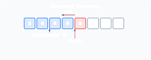
Insertion sort visualisation: building a sorted prefix by inserting elements one at a time

Visual Description

The algorithm maintains two regions: $A[1 \dots j-1]$ is sorted, $A[j \dots n]$ is yet to be processed. At each step, peel off $A[j]$ , walk backwards through the sorted region shifting any larger element right by one position, then drop the key into the gap.

Correctness

Loop invariant: At the start of each FOR iteration, $A[1 \dots j-1]$ consists of the original first $j-1$ elements in sorted order.

Initialisation ( $j=2$ ): $A[1]$ is a single element, trivially sorted.
Maintenance: The WHILE loop shifts all elements greater than Key right by one, preserving sortedness; inserting Key at the correct position extends the sorted prefix by one.
Termination ( $j=n+1$ ): The entire array $A[1 \dots n]$ is sorted.

Complexity Analysis

The running time depends on $t_j$ , the number of WHILE-loop iterations for each $j$ :

$T(n) = a \cdot n + b \cdot (n-1) + d\sum_{j=2}^{n} t_j + e\sum_{j=2}^{n} (t_j - 1)$

Best Case: $\Theta(n)$

Input already sorted. $t_j = 1$ for all $j$ (only the failing comparison, no shifts). $T(n) = pn + q$ .

Worst Case: $\Theta(n^2)$

Input reverse-sorted. $t_j = j$ (shift all previous elements). The comparison count alone is:

$\sum_{j=2}^{n} (j-1) = \frac{n(n-1)}{2} = \Theta(n^2)$

Average Case: $\Theta(n^2)$

On a random permutation, each element moves past roughly half the sorted prefix. The quadratic term carries a factor of $1/2$ but remains $\Theta(n^2)$ .

Properties

Property	Value
In-place	Yes, $O(1)$ extra space
Stable	Yes, equal keys stay in original relative order
Adaptive	Efficient on nearly-sorted data (approaches $O(n)$ )
Online	Can sort items as they arrive

When to Use

Insertion Sort outperforms $\Theta(n \log n)$ algorithms for small $n$ (roughly $n < 50$ ) due to low constant factors and excellent cache locality. It is also ideal for nearly-sorted data or as the base case inside recursive sorts (e.g. switching to Insertion Sort when subarrays fall below a threshold).

Summary

Aspect	Detail
Strategy	Incremental, build sorted prefix
Invariant	$A[1 \dots j-1]$ is sorted
Best case	$\Theta(n)$ , already sorted
Worst case	$\Theta(n^2)$ , reverse-sorted
Average case	$\Theta(n^2)$
Comparisons worst	$n(n-1)/2$
In-place	Yes
Stable	Yes

Binary Insertion Sort

Algorithm

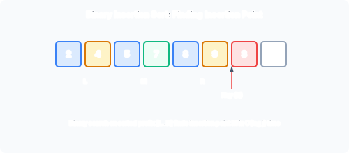
Binary Insertion Sort improves the search step of Insertion Sort by using binary search to find the insertion point, rather than a linear backwards scan. The shifting step remains unchanged.

For each $j$ from 2 to $n$ :

The prefix $A[1 \dots j-1]$ is sorted.
Perform binary search on $A[1 \dots j-1]$ to find the index $k$ where $A[j]$ belongs (the position where all elements before $k$ are $\le A[j]$ ).
Shift $A[k \dots j-1]$ right by one position.
Insert $A[j]$ at position $k$ .

Binary insertion sort: binary search finds insertion point in sorted prefix, then elements shift

Where the Improvement Lies

Standard Insertion Sort uses a linear scan that performs $O(j)$ comparisons to find the insertion point for element $j$ . Binary search performs $O(\log j)$ comparisons. Over all $n$ elements, comparisons drop from $\Theta(n^2)$ to:

$\sum_{j=2}^{n} \log_2 j = \log_2(n!) = \Theta(n \log n)$

Where It Does Not Help

The shifting step still moves up to $j-1$ elements on each insertion. In the worst case, every element must be shifted, requiring:

$\sum_{j=2}^{n} (j-1) = \frac{n(n-1)}{2} = \Theta(n^2)$

movements. Since each shift is a write operation, the total time is still dominated by the $\Theta(n^2)$ shifting cost. The asymptotic running time remains $\Theta(n^2)$ worst case and average case.

Comparison: Standard vs Binary Insertion

Metric	Standard Insertion Sort	Binary Insertion Sort
Comparisons	$\Theta(n^2)$	$\Theta(n \log n)$
Shifts/swaps	$\Theta(n^2)$	$\Theta(n^2)$
Overall time	$\Theta(n^2)$	$\Theta(n^2)$
Best case	$\Theta(n)$	$\Theta(n \log n)$ (binary search still costs $\log j$ each)

The best case actually becomes worse with binary insertion: even on an already-sorted array, binary search still costs $\Theta(\log j)$ comparisons per element, totalling $\Theta(n \log n)$ , whereas standard Insertion Sort gets $\Theta(n)$ .

When Binary Insertion Sort Is Useful

Binary insertion sort helps when:

Comparisons are expensive, and writes are cheap: e.g. sorting strings where each string comparison is costly but copying a pointer (the “shift”) is lightweight.
The data structure supports binary search but not efficient linear scan: e.g. an array where the sorted prefix is conceptually separate from the insertion machinery.

In practice, standard Insertion Sort is usually preferred because its linear scan is cache-friendly and its best case is genuinely linear.

Summary

Aspect	Detail
Search method	Binary search in sorted prefix
Comparison count	$\Theta(n \log n)$
Shift count	$\Theta(n^2)$ worst case
Overall time	$\Theta(n^2)$
Best case	$\Theta(n \log n)$ (worse than standard)
Use case	Expensive comparisons, cheap writes
Compared to standard	Reduces comparisons but does not improve asymptote

Selection Sort

Algorithm

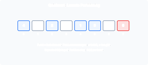
Selection Sort repeatedly finds the minimum element of the unsorted suffix and swaps it with the first unsorted position. For 0-indexed arrays:

For $i = 0$ to $n-2$ :

Find the index $j$ of the minimum element in $A[i \dots n-1]$ .
Swap $A[i]$ with $A[j]$ .

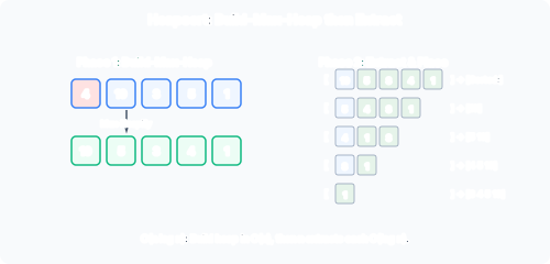
Selection sort: repeatedly select the minimum of what remains and place it at the front

Invariant

At the start of iteration $i$ , the subarray $A[0 \dots i-1]$ contains the $i$ smallest elements of the original array, in sorted order. The remaining elements $A[i \dots n-1]$ are unsorted.

Initialisation ( $i=0$ ): $A[0 \dots -1]$ is empty, trivially sorted.
Maintenance: Appending the next minimum extends the sorted prefix correctly.
Termination ( $i=n-1$ ): $A[0 \dots n-2]$ sorted plus the final element (the largest) at $n-1$ completes the sort.

Complexity: Always $\Theta(n^2)$ Comparisons

Selection Sort performs no early exit. For each $i$ , finding the minimum in the remaining $n-i$ elements requires $n-i-1$ comparisons:

$\sum_{i=0}^{n-2} (n-i-1) = \sum_{k=1}^{n-1} k = \frac{n(n-1)}{2} = \Theta(n^2)$

There is no best-case scenario that reduces comparisons; even if the array is already sorted, every element is still compared. The running time is always $\Theta(n^2)$ comparisons, making it data-insensitive.

Swaps: Only $\Theta(n)$

Each iteration performs exactly one swap, and there are $n-1$ iterations (the last element is automatically in place). Thus the total number of swaps is:

$\text{Swaps} = n-1 = \Theta(n)$

A lower bound theorem shows that any sorting algorithm must perform $\Omega(n)$ swaps in the worst case (consider the input $[2, 3, \ldots, n, 1]$ where every item starts in the wrong place, and each swap touches two items). Selection Sort achieves this lower bound exactly.

Properties

Property	Value
Comparisons	Always $\Theta(n^2)$
Swaps	$\Theta(n)$ (optimal)
In-place	Yes, $O(1)$ space
Stable	No — the swap can jump over equal elements
Data-sensitive	No — same work regardless of input

Why Stability Fails

Consider $[5_a, 5_b, 2]$ . Selection Sort finds 2 as the minimum and swaps it with $5_a$ , producing $[2, 5_b, 5_a]$ . The relative order of $5_a$ and $5_b$ is reversed, so the sort is not stable.

When to Use

Selection Sort is effective when writes are expensive but comparisons are cheap. Each element is written at most twice (once when swapped into the sorted region, once when displaced from the unsorted region), giving $\Theta(n)$ writes total. This is optimal for sorting algorithms.

Summary

Aspect	Detail
Strategy	Repeatedly select minimum, swap to front
Comparisons	$\Theta(n^2)$ , always
Swaps	$\Theta(n)$ , optimal
In-place	Yes
Stable	No
Use case	Expensive writes, cheap comparisons
Lower bound achieved	$\Omega(n)$ swaps

The Comparison-Based Sorting Lower Bound

Statement

Any comparison-based sorting algorithm must perform $\Omega(n \log n)$ comparisons in the worst case to sort $n$ elements.

A comparison-based sort uses only pairwise comparisons ( $\le$ or $>$ ) to determine the relative order of elements. It makes no assumptions about the values (no counting, no hashing, no radix).

Proof via Decision Trees

A decision tree models the behaviour of any comparison-based sort:

Each internal node represents a comparison $A[i] \le A[j]$ , with two outgoing edges (Yes/No).
Each leaf represents a specific permutation of the input — the sorted output.
A path from root to leaf corresponds to the sequence of comparisons made on some input.

For $n$ distinct elements, there are $n!$ possible input permutations. Since the algorithm must be correct for all permutations, the decision tree must have at least $n!$ leaves.

A binary tree of height $h$ has at most $2^h$ leaves. Therefore:

$2^h \ge n!$

Taking logarithms:

$h \ge \log_2(n!)$

Using Stirling’s approximation ( $n! \approx \sqrt{2\pi n}(n/e)^n$ ):

$\log_2(n!) = n \log_2 n - n \log_2 e + O(\log n) = \Omega(n \log n)$

The height $h$ is the number of comparisons on the longest path, so the worst-case number of comparisons is $\Omega(n \log n)$ . $\square$

Implications

MergeSort at $\Theta(n \log n)$ is asymptotically optimal amongst comparison sorts.
HeapSort at $O(n \log n)$ is also optimal.
QuickSort averages $\Theta(n \log n)$ but can degrade to $\Theta(n^2)$ .
No comparison sort can beat $\Omega(n \log n)$ in the worst case.

Lower Bound on Swaps

A separate result: the worst-case number of swaps is $\Omega(n)$ . Consider the input $[2, 3, \ldots, n, 1]$ . Every item is out of position, and each swap moves at most two items to their correct positions. Therefore at least $\lceil n/2 \rceil$ swaps are required. Selection Sort achieves this bound with $\Theta(n)$ swaps.

Comparison Sorts vs Linear-Time Sorts

The $\Omega(n \log n)$ bound applies only to comparison-based sorts. Algorithms that exploit properties of the data can beat this bound:

Sort	Bound	Assumption
Counting Sort	$\Theta(n + k)$	Keys in range $[0, k]$
Radix Sort	$\Theta(d(n + k))$	$d$ -digit numbers
Bucket Sort	$\Theta(n)$ expected	Uniform distribution over $[0, 1)$

These are not comparison-based; they use counting, digit extraction, or hashing.

Summary

Concept	Detail
Lower bound	$\Omega(n \log n)$ comparisons
Proof technique	Decision tree model
Key inequality	$2^h \ge n!$
Stirling’s approx	$\log(n!) \approx n \log n - n \log e$
Optimal sorts	MergeSort, HeapSort (comparison-based)
Swap lower bound	$\Omega(n)$
Exceptions	Linear-time non-comparison sorts

Quicksort: Algorithm

Divide-and-Conquer Structure

Quicksort is a recursive divide-and-conquer sort:

Divide: Choose a pivot element from the array. Partition (rearrange) the array so that all elements $\le$ pivot come before it and all elements $\ge$ pivot come after it.
Conquer: Recursively sort the left and right subarrays (excluding the pivot, which is now in its correct final position).
Combine: Nothing to do — the pivot placement plus recursively sorted subarrays yields a fully sorted array.

Quicksort: pick a pivot, partition around it, recurse on both sides

Lomuto Partitioning

The standard partition scheme (Lomuto) picks the last element as pivot:

x = A[r] (pivot is last element)
i = p - 1 (boundary of ” $\le$ pivot” region)
For j = p to r-1:
If A[j] <= x:
i = i + 1
Swap A[i] and A[j]
Swap A[i+1] and A[r] (place pivot in correct position)
Return i+1 (pivot’s index)

At any point, the array is partitioned as:

$[\, \underbrace{\text{elements} \le x}_{A[p \dots i]} \,|\, \underbrace{\text{elements} > x}_{A[i+1 \dots j-1]} \,|\, \underbrace{\text{unprocessed}}_{A[j \dots r-1]} \,|\, \underbrace{x}_{A[r]} \,]$

Walkthrough Example

Array: $[8, 2, 1, 5, 2, 4]$ with pivot $x = 4$

Step	j	Condition	Action	Result
Init	—	—	i = -1, pivot = 4	$[8, 2, 1, 5, 2, \underline{4}]$
1	0	$8 > 4$	Nothing	$[8, 2, 1, 5, 2, 4]$
2	1	$2 \le 4$	i=0, swap A[0],A[1]	$[2, 8, 1, 5, 2, 4]$
3	2	$1 \le 4$	i=1, swap A[1],A[2]	$[2, 1, 8, 5, 2, 4]$
4	3	$5 > 4$	Nothing	$[2, 1, 8, 5, 2, 4]$
5	4	$2 \le 4$	i=2, swap A[2],A[4]	$[2, 1, 2, 5, 8, 4]$
Final	—	—	swap A[3],A[5]	$[2, 1, 2, \underline{4}, 8, 5]$

Pivot 4 is at index 3. Left subarray $[2, 1, 2]$ and right subarray $[8, 5]$ are recursively sorted.

Hoare Partitioning (Alternative)

Hoare’s scheme uses two pointers moving inward from both ends, swapping out-of-order pairs. It typically performs fewer swaps than Lomuto, and the pivot ends up somewhere in the middle but not necessarily at the returned index.

Pivot Selection Strategies

Strategy	Effect
First element	Simple; worst case on sorted input
Last element	Simple; worst case on reverse-sorted input
Random	Expected $\Theta(n \log n)$ ; eliminates adversarial inputs
Median-of-three	Pivot is median of A[p], A[mid], A[r]; reduces worst-case probability
Median-of-medians	Guaranteed $\Theta(n \log n)$ worst case; high constant factor

The choice of pivot is the single most important factor affecting Quicksort’s performance. A poor pivot (extreme min or max) produces an $n-1$ to 1 split and degrades to $\Theta(n^2)$ . A good pivot (median) gives balanced splits and $\Theta(n \log n)$ .

Properties

Property	Value
In-place	Yes ( $O(\log n)$ stack space for recursion)
Stable	No — partitioning swaps non-adjacent elements
Divide step	$\Theta(n)$ (one scan of subarray)
Combine step	No work required

Quicksort: Analysis

Worst Case: $\Theta(n^2)$

The worst case occurs when the pivot is always the minimum or maximum element of the subarray, producing a split of $0$ and $n-1$ elements. This happens, infamously, when the input is already sorted (or reverse-sorted) with a naive first/last-element pivot choice.

Recurrence:

$T(n) = T(n-1) + T(0) + \Theta(n) = T(n-1) + \Theta(n)$

Using the substitution method:

$T(n) = T(n-1) + kn = (T(n-2) + k(n-1)) + kn = \dots = \Theta(1) + k\sum_{i=1}^{n} i = \Theta(n^2)$

Even a constant-sized split-off (e.g. consistently producing a subarray of size $x$ and $n-x-1$ for constant $x$ ) still yields $\Theta(n^2)$ , because the recurrence becomes $T(n) = T(n-c) + \Theta(n)$ .

Best Case: $\Theta(n \log n)$

If the pivot always splits the array exactly in half:

$T(n) = 2T(n/2) + \Theta(n)$

By the Master Theorem (Case 2, $a=2, b=2, f(n)=\Theta(n) = \Theta(n^{\log_2 2})$ ):

$T(n) = \Theta(n \log n)$

Ratio Splits Also Give $\Theta(n \log n)$

A split of $1/4$ to $3/4$ still produces $\Theta(n \log n)$ . The recursion tree has depth $\log_{4/3} n$ on the longest path and $\log_4 n$ on the shortest, with at most $kn$ work per level. In both cases:

$T(n) \le kn \cdot \log_{4/3} n = \Theta(n \log n)$

An ratio split (any constant fraction on both sides, no matter how unbalanced) guarantees $\Theta(n \log n)$ . Only constant-sized splits degrade to $\Theta(n^2)$ .

Average Case: $\Theta(n \log n)$

Assuming random pivot selection (all permutations equally likely), the expected number of comparisons is approximately $2n \ln n \approx 1.39 \, n \log_2 n$ .

Intuition: any two elements $z_i$ and $z_j$ (with $i < j$ in sorted order) are compared if and only if one of them is chosen as a pivot before any element between them in sorted order. The probability they are compared is $\frac{2}{j-i+1}$ . Summing over all pairs:

$\mathbb{E}[\text{comparisons}] = \sum_{i=1}^{n-1} \sum_{j=i+1}^{n} \frac{2}{j-i+1} = \sum_{i=1}^{n-1} \sum_{k=2}^{n-i+1} \frac{2}{k} \le 2n \sum_{k=1}^{n} \frac{1}{k} \approx 2n \ln n + O(n)$

Thus the expected running time is $\Theta(n \log n)$ .

Comparison with MergeSort

Property	Quicksort	MergeSort
Worst case	$\Theta(n^2)$	$\Theta(n \log n)$
Average case	$\Theta(n \log n)$	$\Theta(n \log n)$
Extra space	$O(\log n)$ (stack)	$\Theta(n)$ (merge arrays)
Stable	No	Yes
Cache behaviour	Excellent (in-place, sequential access)	Good but external merge requires extra memory

Despite the $\Theta(n^2)$ worst case, Quicksort is often faster than MergeSort in practice because of low constant factors and cache-friendly memory access patterns. The worst case can be mitigated by random pivot selection or median-of-three.

Summary

Case	Running Time	Condition
Best	$\Theta(n \log n)$	Pivot always splits evenly
Average	$\Theta(n \log n)$	Random pivot; expected ${\sim}2n \ln n$ comparisons
Worst	$\Theta(n^2)$	Pivot always min or max
Ratio split	$\Theta(n \log n)$	Any constant fraction split
Constant split	$\Theta(n^2)$	Splitting off constant-size chunk
Key insight	Unbalanced but proportional splits are fine; constant-remainder splits are disastrous

Mergesort

Algorithm

Mergesort is a classic divide-and-conquer sorting algorithm:

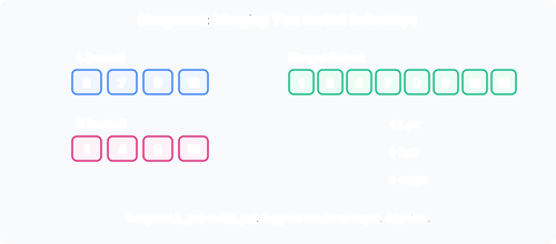
Divide: Split the array into two halves of (roughly) equal size.
Conquer: Recursively sort each half.
Combine: Merge the two sorted halves into a single sorted array.

Mergesort: divide array into halves, recursively sort, then merge

Merge Procedure

Given two sorted subarrays $L$ and $R$ , use two pointers $i$ and $j$ :

Initialise $i=1$ , $j=1$ (pointing to the start of each subarray).
For $k = 1$ to $|L| + |R|$ :
If $L[i] \le R[j]$ : place $L[i]$ into output, increment $i$ .
Else: place $R[j]$ into output, increment $j$ .
If one subarray is exhausted, copy the remainder of the other.

A common trick: append a sentinel $\infty$ to both subarrays so neither is ever exhausted before the loop ends.

Walkthrough Example

Input: $[9, 102, 10, -7, 64, 18]$

Split:                [9, 10, 102, -7, 64, 18]
                     /                          \
           [9, 10, 102]                    [-7, 64, 18]
          /            \                  /             \
     [9]                [10, 102]     [-7]              [64, 18]
   (base)             /       \     (base)            /        \
                 [10]          [102]              [64]          [18]
                (base)        (base)            (base)        (base)

Merge up: [9] + [10, 102] -> [9, 10, 102]
          [64] + [18] -> [18, 64]   (sorted merge)
          [-7] + [18, 64] -> [-7, 18, 64]
          [9, 10, 102] + [-7, 18, 64] -> [-7, 9, 10, 18, 64, 102]

Analysis

Recurrence

Let $T(n)$ be the cost of sorting $n$ elements:

$T(n) = \begin{cases} \Theta(1) & \text{if } n = 1 \\ 2T(n/2) + \Theta(n) & \text{if } n > 1 \end{cases}$

The $\Theta(n)$ term covers both the array copying for the subarrays and the merge comparison loop.

Closed Form via Substitution

Unwinding the recurrence:

$T(n) = 2T(n/2) + kn = 2[2T(n/4) + k n/2] + kn = 4T(n/4) + 2kn$

After $\log_2 n$ substitutions:

$T(n) = nT(1) + kn \log_2 n = \Theta(n \log n)$

Via Master Theorem

$a = 2$ , $b = 2$ , $f(n) = \Theta(n)$ . Compute $n^{\log_b a} = n^{\log_2 2} = n$ . Since $f(n) = \Theta(n^{\log_b a})$ , Case 2 applies:

$T(n) = \Theta(n^{\log_b a} \cdot \log n) = \Theta(n \log n)$

The Call Tree Method

At the top level, merge costs $kn$ . At the next level, two merges each cost $k n/2$ , totalling $kn$ . Each of the $\log_2 n + 1$ levels contributes exactly $kn$ , so $T(n) = kn(\log_2 n + 1) = \Theta(n \log n)$ .

Properties

Property	Value
Worst case	$\Theta(n \log n)$
Average case	$\Theta(n \log n)$
Best case	$\Theta(n \log n)$
Stable	Yes — merge preserves order of equal keys
In-place	No (standard); $\Theta(n)$ extra space
Data-sensitive	No — always $\Theta(n \log n)$
Non-integer $n$	$T(n) = T(\lceil n/2 \rceil) + T(\lfloor n/2 \rfloor) + \Theta(n)$ , same solution

Variations

Bottom-up merge sort: Iterative, merging pairs of size 1, then 2, then 4, etc. Useful for linked lists where splitting is $O(1)$ .
Natural merge sort: Exploits existing runs (sorted subsequences) in the input; can approach $O(n)$ on nearly-sorted data.
In-place merge sort: The merge step can be made in-place with clever data movement, but the constant factor becomes large and practical implementations use the extra space.

Summary

Aspect	Detail
Strategy	Divide and conquer
Recurrence	$T(n) = 2T(n/2) + \Theta(n)$
Solution	$\Theta(n \log n)$
Master Theorem	Case 2: $a=2, b=2, f(n)=\Theta(n)$
Space	$\Theta(n)$ extra
Stable	Yes
Optimal	Yes — matches $\Omega(n \log n)$ lower bound

Heaps and Heapsort

The binary heap data structure, heapify, building a heap in linear time, and the heapsort algorithm

The Binary Heap Structure

Definition

A (binary) max-heap is a complete binary tree satisfying the heap property: the value at every node is greater than or equal to the values of its children. A min-heap reverses this: every node is less than or equal to its children.

Two defining properties:

Structural property: The tree is complete — every level except possibly the bottom is full, and the bottom level is filled from left to right.
Ordering property: Parent $\ge$ children (max-heap) or Parent $\le$ children (min-heap).

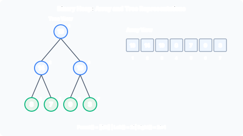
A max-heap showing parent values greater than or equal to children, and the corresponding array layout

Array Representation

The complete binary tree structure enables a compact array representation. Using 1-indexed arrays:

Root at $A[1]$ .
Left child of node $i$ : $A[2i]$ .
Right child of node $i$ : $A[2i + 1]$ .
Parent of node $i$ : $A[\lfloor i/2 \rfloor]$ .

The root has no parent ( $\lfloor 1/2 \rfloor = 0$ ). A child is absent when $2i$ or $2i + 1$ exceeds A.heap_size (which may be less than A.length since the heap may occupy only a prefix of the array).

Height of a Heap

A heap with $n$ nodes has height $h = \lfloor \log_2 n \rfloor$ . The number of nodes at level $k$ is at most $2^k$ , and the deepest leaf is at level $h$ .

For $n=6$ : $h = \lfloor \log_2 6 \rfloor = \lfloor 2.58 \rfloor = 2$ .
For $n=15$ : $h = \lfloor \log_2 15 \rfloor = 3$ (a perfect binary tree).

Operations that traverse from root to leaf (or leaf to root) are bounded by the height, giving $O(\log n)$ time.

Heap vs Binary Search Tree

Property	Heap	BST
Left-right ordering	None; only parent-child inequality	Left subtree < root < right subtree
Structure	Complete tree	No structural guarantee (can be degenerate)
Finding min/max	$O(1)$ — always at root	$O(h)$ — traverse to leftmost/rightmost
Searching	$O(n)$ — must scan	$O(h)$ if balanced
In-order traversal	Not meaningful	Produces sorted order
Use case	Priority queue, Heapsort	Dictionary, ordered map

The heap is a semi-structure: cheaper to maintain than a fully ordered structure, yet sufficient for repeatedly extracting the largest (or smallest) element.

Semi-Structured Nature

In a max-heap of $n$ elements:

The largest is at exactly one place: the root.
The second largest is in one of two places: the root’s children.
The third largest is in one of three places: the other root child, or either child of the second largest.

This “partial-sort” property is what makes heap operations $O(\log n)$ rather than the $O(n \log n)$ cost of full sorting.

Summary

Property	Detail
Structure	Complete binary tree, array representation
Parent at $i$	$\lfloor i/2 \rfloor$
Left child at $i$	$2i$
Right child at $i$	$2i + 1$
Height	$\lfloor \log_2 n \rfloor$
Heap property (max)	$A[i] \ge A[2i], A[2i+1]$
Heap vs BST	Heap: weak order, strong structure; BST: strong order, weak structure

Heap Operations

All max-heap operations run in $O(\log n)$ time, where $n$ is the number of elements in the heap. Each operation works by traversing a single path from root to leaf (or leaf to root), bounded by the heap height $\lfloor \log_2 n \rfloor$ .

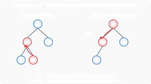
Max-Heapify (Bubble-Down)

Purpose: Restore the max-heap property at node $i$ , assuming the subtrees rooted at $i$ ‘s children are already valid max-heaps.

Algorithm:

Let $l = 2i$ , $r = 2i + 1$ .
Set largest to $i$ if $A[i] \ge A[l]$ (or $l$ exceeds heap size), else to $l$ .
If $r$ is within heap and $A[r] > A[\text{largest}]$ , set largest to $r$ .
If largest $\ne i$ , swap $A[i]$ and $A[\text{largest}]$ , then recursively call Max-Heapify on largest.

Time: $O(\log n)$ — each swap moves down one level, at most the height of the heap.

Max-heapify: compare node with children, swap with larger child, recurse down

Walkthrough

Starting with a heap violation at the root: $A = [4, 14, 10, 8, 7, 9, 3, 2, 1]$ (node $A[1] = 4$ , children $14$ and $10$ ):

Step	Current node	Children	Largest	Action
1	$4$ at index 1	$14$ , $10$	$14$ at index 2	Swap 4 and 14
2	$4$ at index 2	$8$ , $7$	$8$ at index 4	Swap 4 and 8
3	$4$ at index 4	$2$ , $1$	$4$ at index 4	No swap; done

Result: $[14, 8, 10, 4, 7, 9, 3, 2, 1]$ — a valid max-heap.

Insert (Bubble-Up)

Purpose: Insert a new key into the heap.

Algorithm:

Increment heap_size; place the new key at $A[\text{heap\_size}]$ .
Set $j = \text{heap\_size}$ .
While $j > 0$ and $A[j] > A[\text{parent}(j)]$ :
Swap $A[j]$ and $A[\text{parent}(j)]$ .
$j = \text{parent}(j)$ .

Time: $O(\log n)$ — at most one swap per level up to the root.

Extract-Max

Purpose: Remove and return the largest element (the root).

Algorithm:

If the heap is empty, error.
Store $A[1]$ (the maximum).
Swap $A[1]$ with $A[\text{heap\_size}]$ .
Decrement heap_size.
Call Max-Heapify on the root (index 1).
Return stored maximum.

Time: $O(\log n)$ — constant work plus one Max-Heapify call.

The swap with the last element preserves the structural property (only the rightmost bottom element can be removed without breaking completeness). The heap property is fixed by bubbling the new root downwards.

Increase-Key (Bubble-Up)

Purpose: Increase the value of a key at position $i$ , then restore the heap property by moving it upward.

Algorithm:

If new value < current value, error.
Set $A[i]$ to new value.
While $i > 1$ and $A[i] > A[\text{parent}(i)]$ :
Swap $A[i]$ and $A[\text{parent}(i)]$ .
$i = \text{parent}(i)$ .

Time: $O(\log n)$ .

Max-Peek

Simply return $A[1]$ in $O(1)$ time. No modification to the heap.

Operations Summary

Operation	Purpose	Time	Method
Max-Heapify	Fix a single violation	$O(\log n)$	Bubble down
Insert	Add new element	$O(\log n)$	Add at end, bubble up
Extract-Max	Remove and return max	$O(\log n)$	Swap with last, bubble down
Increase-Key	Update to larger value	$O(\log n)$	Update, bubble up
Max-Peek	View maximum	$O(1)$	Read $A[1]$

All operations rely on the heap height being $\lfloor \log_2 n \rfloor$ , ensuring each upward or downward traversal touches at most $O(\log n)$ nodes.

Building a Heap in Linear Time

Naive Build: $\Theta(n \log n)$

Inserting $n$ elements one by one, each costing $O(\log n)$ , gives $\Theta(n \log n)$ total. This is the obvious approach but not optimal.

Linear-Time Build: Bottom-Up Heapify

A more efficient method calls Max-Heapify on all non-leaf nodes, working bottom-up from $\lfloor n/2 \rfloor$ down to 1:

Build-Max-Heap(A):
  A.heap_size = A.length
  for i = floor(A.length / 2) downto 1:
    Max-Heapify(A, i)

The key insight: leaves (indices $\lfloor n/2 \rfloor + 1$ to $n$ ) are already 1-element max-heaps, so they need no work. Starting from the last non-leaf node and working upward ensures that when Max-Heapify is called on node $i$ , both subtrees of $i$ are already valid heaps.

Correctness

Loop invariant: At the start of each iteration, every node index $> i$ is the root of a valid max-heap.

Initialisation ( $i = \lfloor n/2 \rfloor$ ): All nodes $> \lfloor n/2 \rfloor$ are leaves, trivially heaps.
Maintenance: Max-Heapify fixes node $i$ ; after the call, $i$ is also a heap root. Moving to $i-1$ preserves the invariant.
Termination ( $i = 0$ ): All nodes, including the root (index 1), are valid heaps.

Analysis: Why $O(n)$

The cost of Max-Heapify at node $i$ is proportional to the height of node $i$ , i.e. the number of levels below it. At level $h$ from the bottom (height $h$ ), there are at most $\lceil n / 2^{h+1} \rceil$ nodes, and each Max-Heapify costs $O(h)$ . Summing over all levels:

$T(n) \le \sum_{h=0}^{\lfloor \log n \rfloor} \left\lceil \frac{n}{2^{h+1}} \right\rceil \cdot c h \le c \cdot \frac{n}{2} \sum_{h=0}^{\infty} \frac{h}{2^{h-1}}$

The infinite sum converges: $\sum_{h=0}^{\infty} h/2^{h} = 2$ . Therefore:

$T(n) = O(n)$

Concrete Calculation

For $n = 15$ (a perfect heap), the tree has 4 levels:

Level (from leaf)	Height $h$	Nodes at this level	Work per node	Total work
0 (leaves)	0	8	0	0
1	1	4	$c$	$4c$
2	2	2	$2c$	$4c$
3 (root)	3	1	$3c$	$3c$

Total: $11c$ , whilst $n \log n$ would be $15 \times 3.9c \approx 59c$ . The linear-time build is substantially faster.

Step-by-Step Example

Input: $A = [4, 1, 3, 2, 16, 9, 10, 14, 8, 7]$ ( $n=10$ )

First non-leaf: $\lfloor 10/2 \rfloor = 5$ , value $16$ .

Initial array as tree:          After Build-Heap (final):
          4                                 16
      /       \                          /      \
     1         3                       14        10
   /   \     /   \                   /   \     /    \
  2    16   9     10                8     7   9      3
 / \   /                          / \   /
14  8 7                          2   4  1

Step	$i$	Action	Key effect
1	5	Max-Heapify on node with value 16	Already a heap (16 > 7)
2	4	Max-Heapify on node with value 2	Swap 2 with 14; $[14, 8]$ heap
3	3	Max-Heapify on node with value 3	Swap 3 with 10; $[10, 9]$ heap
4	2	Max-Heapify on node with value 1	Swap 1 with 16, then 1 with 7; heap
5	1	Max-Heapify on node with value 4	Swap 4 with 16, then 4 with 14, then 4 with 8

Final heap: $[16, 14, 10, 8, 7, 9, 3, 2, 4, 1]$ .

Summary

Aspect	Detail
Naive build	Insert $n$ elements: $\Theta(n \log n)$
Efficient build	Bottom-up heapify: $\Theta(n)$
Starting index	$\lfloor n/2 \rfloor$ (last non-leaf)
Why $O(n)$	Most nodes (leaves) cost $O(0)$ ; higher nodes are few
Series sum	$\sum h / 2^{h}$ converges to 2
Key insight	Work is proportional to height, not depth

Heapsort

Algorithm

Heapsort sorts an array in two phases:

Phase 1: Build a max-heap from the input array in $O(n)$ time.

Phase 2: Repeatedly extract the maximum and place it at the end:

Build-Max-Heap( $A$ ).
For $i = A.\text{length}$ down to 2:
Swap $A[1]$ (the maximum) with $A[i]$ .
Decrement heap_size (excludes the sorted suffix).
Max-Heapify( $A$ , 1).

Heapsort: build max-heap, then repeatedly extract max to build sorted suffix

After each iteration, $A[1 \dots i-1]$ is a max-heap and $A[i \dots n]$ contains the largest $n-i+1$ elements in sorted order. When $i$ reaches $2$ , the entire array is sorted in ascending order (assuming a max-heap; for descending order, use a min-heap).

Walkthrough

Input: $[1, 9, 3, 4, 2, 7, 6, 5, 8]$

Phase 1 (Build-Heap): $[1, 9, 3, 4, 2, 7, 6, 5, 8] → [9, 8, 7, 5, 2, 3, 6, 1, 4]$ (max-heap)

Phase 2 (Extract-Max loop):
  i=9: swap 9 ⇄ 4, heapify → heap [8,5,7,1,2,3,6,4 | 9]
  i=8: swap 8 ⇄ 4, heapify → heap [7,5,6,1,2,3,4 | 8, 9]
  i=7: swap 7 ⇄ 4, heapify → heap [6,5,3,1,2,4 | 7, 8, 9]
  i=6: swap 6 ⇄ 4, heapify → heap [5,4,3,1,2 | 6, 7, 8, 9]
  i=5: swap 5 ⇄ 2, heapify → heap [4,2,3,1 | 5, 6, 7, 8, 9]
  i=4: swap 4 ⇄ 1, heapify → heap [3,2,1 | 4, 5, 6, 7, 8, 9]
  i=3: swap 3 ⇄ 1, heapify → heap [2,1 | 3, 4, 5, 6, 7, 8, 9]
  i=2: swap 2 ⇄ 1, heapify → heap [1 | 2, 3, 4, 5, 6, 7, 8, 9]

Final: [1, 2, 3, 4, 5, 6, 7, 8, 9]

Complexity Analysis

Phase 1 (Build-Max-Heap): $\Theta(n)$ as proved earlier.

Phase 2: $n-1$ iterations, each calling Max-Heapify on the root of a shrinking heap. Max-Heapify on a heap of size $k$ costs $O(\log k)$ . Summing:

$T(n) = \Theta(n) + \sum_{k=2}^{n} O(\log k) = \Theta(n) + O(\log(n!))$

Using Stirling’s approximation: $\log(n!) \le n \log n - n + O(\log n)$ . Therefore:

$T(n) = O(n \log n)$

This bound is worst-case. Heapsort never degrades to $\Theta(n^2)$ , unlike Quicksort.

In-Place Property

Heapsort uses only $O(1)$ extra space beyond the input array (a few variables for indices and the temporary for swaps). The heap is stored within the same array as the sorted output, separated by the heap_size boundary. This is achieved by using the suffix of the array for the sorted region and the prefix for the heap.

Cache Performance

Heapsort’s in-place nature comes at a cost: Max-Heapify jumps between array positions at powers of 2 ( $i \to 2i \to 4i \to \dots$ ), which are far apart in memory for large indices. This results in poor cache locality compared to Quicksort (which scans contiguously during partitioning) and MergeSort (which merges contiguously). In practice, Heapsort is often slower than Quicksort for moderate $n$ , despite its superior worst-case guarantee.

Comparison with Other Sorts

Sort	Worst Case	Average Case	In-place	Stable
Heapsort	$O(n \log n)$	$O(n \log n)$	Yes	No
MergeSort	$\Theta(n \log n)$	$\Theta(n \log n)$	No ( $\Theta(n)$ )	Yes
Quicksort	$\Theta(n^2)$	$\Theta(n \log n)$	Yes	No
Insertion Sort	$\Theta(n^2)$	$\Theta(n^2)$	Yes	Yes

Summary

Phase	Cost	Description
Build-Heap	$\Theta(n)$	Bottom-up max-heapify
Extract loop	$O(n \log n)$	$n-1$ extractions, each $O(\log k)$
Total	$O(n \log n)$	Worst-case guarantee
Space	$O(1)$	In-place via array prefix/suffix split
Stable	No	Swaps non-adjacent elements
Cache	Poor	Non-local memory access pattern
Advantage	Good worst case, in-place
Disadvantage	Slower constant factors, poor cache

Linear-Time Sorts

Counting sort, radix sort, bucket sort, stability, the decision-tree lower bound, and order statistics

Counting Sort

Overview

Counting sort sorts $n$ integers drawn from a known range $[0, k]$ . It is not a comparison sort, so it evades the $\Omega(n \log n)$ lower bound. Instead, it counts occurrences of each value, computes cumulative counts to determine output positions, and places each element directly into its correct sorted position.

Running time is $\Theta(n + k)$ ; space is $\Theta(n + k)$ . Counting sort is stable. It is practical linear time only when $k = O(n)$ .

Algorithm

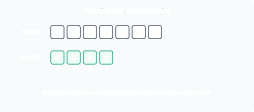
Counting sort diagram

Given input array A of length $n$ and maximum value $k$ :

Allocate a count array C[0..k], initialise all entries to 0.
For each element $v$ in A, increment C[v].
Convert C to cumulative counts: for $i = 1$ to $k$ , set C[i] = C[i] + C[i-1]. Now C[i] is the number of elements $\le i$ .
Allocate output array B[1..n]. Iterate through A from right to left (to preserve stability): for each $v = A[j]$ , place it at B[C[v]], then decrement C[v].

The right-to-left pass in step 4 is what guarantees stability: when duplicate values exist, the element appearing later in the input is placed later in the output.

Worked Example

Sort A = [2, 5, 3, 0, 2, 3, 0, 3] with $k = 5$ .

Step 1: Count occurrences

$i$	0	1	2	3	4	5
`C[i]`	2	0	2	3	0	1

Step 2: Cumulative counts

$i$	0	1	2	3	4	5
`C[i]`	2	2	4	7	7	8

Interpretation: there are 2 elements $\le 0$ , 2 elements $\le 1$ , 4 elements $\le 2$ , etc. So the value 2 will occupy output positions 3 and 4 (1-indexed: C[2] = 4, then decrement yields 3 for next occurrence).

Step 3: Place elements (right to left)

$A[8] = 3$ : C[3] = 7 → B[7] = 3, C[3] = 6
$A[7] = 0$ : C[0] = 2 → B[2] = 0, C[0] = 1
$A[6] = 3$ : C[3] = 6 → B[6] = 3, C[3] = 5
$A[5] = 2$ : C[2] = 4 → B[4] = 2, C[2] = 3
$A[4] = 0$ : C[0] = 1 → B[1] = 0, C[0] = 0
$A[3] = 3$ : C[3] = 5 → B[5] = 3, C[3] = 4
$A[2] = 5$ : C[5] = 8 → B[8] = 5, C[5] = 7
$A[1] = 2$ : C[2] = 3 → B[3] = 2, C[2] = 2

Output: B = [0, 0, 2, 2, 3, 3, 3, 5]. Notice that the two 0s preserve their original relative order, as do the two 2s and three 3s. The sort is stable.

Complexity Analysis

Step	Cost
Initialise `C[0..k]`	$\Theta(k)$
Count occurrences	$\Theta(n)$
Cumulative counts	$\Theta(k)$
Place elements	$\Theta(n)$
Total	$\Theta(n + k)$

Space: $\Theta(n + k)$ for the output array and count array. Counting sort is not in-place.

When Is It Linear?

If $k = O(n)$ , then $\Theta(n + k) = \Theta(n)$ . This is the practical regime. If $k$ is much larger than $n$ (e.g. sorting a handful of 64-bit integers), then counting sort is $\Theta(k)$ -dominated and wastes both time and space.

Why It Beats the Lower Bound

The $\Omega(n \log n)$ lower bound applies only to comparison-based sorting. Counting sort never compares elements against each other; it inspects the numerical value of each key directly and uses that value as an array index. This is not a valid operation in the comparison model.

Stability

Counting sort is stable because we iterate the input from right to left when placing elements. The last occurrence of a value in the original array is placed at the rightmost available position for that value in the output, preserving relative order amongst equal keys.

Summary

Property	Value
Type	Non-comparison, integer sort
Worst-case time	$\Theta(n + k)$
Space	$\Theta(n + k)$
Stable	Yes
In-place	No
Practical when	$k = O(n)$
Beats $\Omega(n \log n)$	Yes (not comparison-based)

Radix Sort

Overview

Radix sort sorts integers digit by digit, starting from the least significant digit (LSD). It uses a stable auxiliary sort (typically counting sort) on each digit position, proceeding from right to left. If each digit lies in the range $[0, k-1]$ and there are $d$ digits, the running time is $\Theta(d(n + k))$ .

The algorithm relies critically on the stability of the per-digit sort: when we sort by a more significant digit, equal digits in that position preserve the ordering established by all less significant digits.

Algorithm (LSD Radix Sort)

Radix sort diagram

for i = 1 to d:
    stably sort array A on digit i

Digit 1 is the least significant digit (units). Each pass uses counting sort with $k$ being the radix (base) of the digit — typically $k = 10$ for decimal or $k = 256$ for byte-based sorting.

Worked Example

Sort [170, 45, 75, 90, 802, 24, 2, 66] by decimal digits ( $d = 3$ , pad with leading zeros: [170, 045, 075, 090, 802, 024, 002, 066]).

Pass 1: Sort by units digit (digit 1) Sorting stably by the last digit groups by units: 170(0), 090(0), 802(2), 002(2), 024(4), 045(5), 075(5), 066(6).

Result: [170, 090, 802, 002, 024, 045, 075, 066]

Pass 2: Sort by tens digit (digit 2) Stable sort by tens digit: 802(0), 002(0), 024(2), 045(4), 066(6), 170(7), 075(7), 090(9).

Result: [802, 002, 024, 045, 066, 170, 075, 090]

Pass 3: Sort by hundreds digit (digit 3) Stable sort by hundreds: 002(0), 024(0), 045(0), 066(0), 075(0), 090(0), 170(1), 802(8).

Result: [2, 24, 45, 66, 75, 90, 170, 802]

Sorted. Notice that 170 and 075 both had tens digit 7; stability preserved their order from the units pass (0 before 5, so 170 before 75). Similarly, 802 and 002 both had hundreds digit 0; stability preserved the tens-digit ordering.

Why LSD Works

After pass 1, the array is sorted by the least significant digit. Pass 2 sorts by the next digit; because the sort is stable, when two elements have the same value in digit 2, they remain in the order determined by pass 1 (i.e. by digit 1). By induction, after $d$ passes the array is fully sorted.

If the per-digit sort were unstable, a later pass could scramble the ordering established by earlier passes. Stability is therefore essential to radix sort’s correctness.

Complexity Analysis

For $n$ numbers with $d$ digits each, using counting sort for each digit:

Each counting sort pass: $\Theta(n + k)$
$d$ passes: $\Theta(d(n + k))$

For 32-bit integers, choosing bytes as digits gives $d = 4$ , $k = 256$ . Then $\Theta(4(n + 256)) = \Theta(n)$ . Radix sort is a linear-time sort for fixed-width integers.

Historical Note

Radix sort was used by Herman Hollerith in his 1890 US Census tabulating machine. Punch cards were physically sorted into bins (digit buckets) and gathered, one digit column at a time. The IBM 83 Card Sorter (1955) sorted 1000 cards per minute using the same principle.

Comparison with Other Linear Sorts

Sort	Assumption	Time
Counting sort	Keys in $[0, k]$ , $k = O(n)$	$\Theta(n + k)$
Radix sort	$d$ digits, each $0..k-1$	$\Theta(d(n + k))$
Bucket sort	Uniform distribution in $[0, 1)$	$\Theta(n)$ average

Radix sort generalises counting sort to larger key ranges by treating keys as composed of smaller-range digits.

Summary

Property	Value
Type	Non-comparison, digit-by-digit sort
Worst-case time	$\Theta(d(n + k))$
Space	Depends on underlying stable sort
Stable	Yes (if digit sort is stable)
Practical for	Fixed-width integers, strings
Beats $\Omega(n \log n)$	Yes (not comparison-based)

Bucket Sort

Overview

Bucket sort distributes $n$ inputs into $k$ buckets according to their key range, sorts each bucket individually (typically with insertion sort), and concatenates the buckets in order. It assumes the input is drawn uniformly from a known interval. Under this assumption, each bucket receives approximately $n/k$ elements and the average-case running time is $\Theta(n)$ .

Worst-case running time is $\Theta(n^2)$ if all elements fall into one bucket, since insertion sort on $n$ elements is $\Theta(n^2)$ .

Algorithm

Bucket sort diagram

For input in the range $[0, 1)$ :

Create $n$ empty buckets (linked lists or arrays).
For each element $x$ , insert it into bucket $\lfloor n \cdot x \rfloor$ .
Sort each bucket (e.g. with insertion sort).
Concatenate buckets in order (0, 1, …, $n-1$ ).

The bucket index $\lfloor n \cdot x \rfloor$ maps the uniform $[0, 1)$ range onto $n$ equal-width intervals.

Worked Example

Input: $[0.78, 0.17, 0.39, 0.26, 0.72, 0.94, 0.21, 0.12, 0.23, 0.68]$ , $n = 10$ .

Step 2: Distribute into buckets ( $\lfloor 10 \cdot x \rfloor$ ):

Bucket	Range	Elements
0	$[0, 0.1)$	—
1	$[0.1, 0.2)$	0.17, 0.12
2	$[0.2, 0.3)$	0.26, 0.21, 0.23
3	$[0.3, 0.4)$	0.39
4	$[0.4, 0.5)$	—
5	$[0.5, 0.6)$	—
6	$[0.6, 0.7)$	0.68
7	$[0.7, 0.8)$	0.78, 0.72
8	$[0.8, 0.9)$	—
9	$[0.9, 1.0)$	0.94

Step 3: Sort each bucket (insertion sort):

Bucket 1: $[0.12, 0.17]$
Bucket 2: $[0.21, 0.23, 0.26]$
Bucket 3: $[0.39]$
Bucket 6: $[0.68]$
Bucket 7: $[0.72, 0.78]$
Bucket 9: $[0.94]$

Step 4: Concatenate: $[0.12, 0.17, 0.21, 0.23, 0.26, 0.39, 0.68, 0.72, 0.78, 0.94]$

Complexity Analysis

Distribution into $n$ buckets: $\Theta(n)$ . Sorting each bucket: let $n_i$ be the number of elements in bucket $i$ . Insertion sort on bucket $i$ costs $O(n_i^2)$ . Total:

$T(n) = \Theta(n) + \sum_{i=0}^{n-1} O(n_i^2)$

Under the uniform distribution assumption, the expected value of $n_i^2$ is $2 - 1/n$ , giving $T(n) = \Theta(n) + n \cdot O(2 - 1/n) = \Theta(n)$ .

If the uniformity assumption fails and all $n$ elements land in one bucket, insertion sort on that bucket costs $\Theta(n^2)$ , which is the worst case.

Comparison with Counting Sort and Radix Sort

Sort	Assumption	Average	Worst
Counting sort	Integer keys in $[0, k]$	$\Theta(n + k)$	$\Theta(n + k)$
Radix sort	$d$ -digit integers	$\Theta(d(n + k))$	$\Theta(d(n + k))$
Bucket sort	Uniform real keys in $[0, 1)$	$\Theta(n)$	$\Theta(n^2)$

Bucket sort is the only one of the three whose worst case is quadratic. Its average-case speed depends on the uniform-distribution assumption, whereas counting and radix sort guarantee their bounds for all inputs satisfying their range constraints.

Practical Use

Bucket sort is most useful when input is known to be uniformly distributed — for example, hashing a uniform key space into buckets. In practice, it is often combined with other techniques (e.g. using a better sort within buckets, or using it as one phase of a hybrid algorithm).

Summary

Property	Value
Type	Non-comparison, distribution sort
Average time	$\Theta(n)$
Worst-case time	$\Theta(n^2)$
Space	$\Theta(n)$ for buckets
Stable	Depends on bucket sort
Assumption	Uniform distribution of keys
Beats $\Omega(n \log n)$	Yes on average (not comparison-based)

Stability of Sorting Algorithms

Definition

A sorting algorithm is stable if, for any two elements with equal sort keys, their relative order in the input is preserved in the output. In other words, if $A[i] = A[j]$ and $i < j$ , then after sorting, the element originally at $i$ appears before the element originally at $j$ .

Stability is about the behaviour with respect to duplicate keys; it says nothing about the algorithm’s running time.

Which Sorts Are Stable

Algorithm	Stable?	Reason
Insertion sort	Yes	Places each element into its correct sorted position without jumping over equal elements
Selection sort	No	Swapping the minimum into position can leap over equal elements, changing their relative order
Mergesort	Yes	Merge takes from the left subarray when keys are equal, preserving input order
Quicksort	No	Partitioning swaps elements arbitrarily; equal keys can cross each other
Heapsort	No	Heap operations (reheapify, extract) do not preserve relative order of equal keys
Counting sort	Yes	Iterates from right to left when placing output, preserving rightmost-later ordering
Radix sort	Depends	Stable if the underlying digit sort is stable (typically counting sort)
Bucket sort	Depends	Stable if the sort used within each bucket is stable and concatenation is ordered

Why Stability Matters

Multi-key Sorting

Suppose we want to sort student records first by exam mark (descending) and then alphabetically by surname for students with the same mark. Using a stable sort:

Sort by surname (any sort works for this pass).
Stably sort by mark.

After step 2, students with equal marks remain in surname order from step 1. If the mark sort were unstable, the alphabetical ordering could be destroyed.

This technique generalises: to sort by $m$ keys in priority order (least significant first), use $m$ stable sorts. This is sometimes called the “stable sort composition” property.

Radix Sort

Radix sort depends fundamentally on stability. Each digit pass must preserve the ordering established by less significant digits. An unstable digit sort would scramble the work of previous passes, making the algorithm incorrect.

If you only have access to an unstable sort and need stability, you can extend the sort key to include the original index as a tiebreaker: (original_key, original_index). This guarantees uniqueness and simulates stability, at the cost of $\Theta(n)$ extra space for the extended records.

Counterexample: Unstable Quicksort

Given [(3, A), (3, B)] where A and B are the original order:

Choose pivot = 3 (the last element, (3, B)).
All other elements are $\le$ pivot, so they land left of pivot.
The partition may swap (3, A) with itself or rearrange arbitrarily.
Output might be [(3, B), (3, A)], violating stability.

Summary

Property	Value
Stable sorts	Insertion, Mergesort, Counting sort, (some) Radix
Unstable sorts	Selection, Quicksort, Heapsort
Key uses	Multi-key sorting, radix sort, duplicate-sensitive applications
Emulating stability	Extend key with original index as tiebreaker

The Decision-Tree Lower Bound Proof

Overview

Any comparison-based sorting algorithm must perform $\Omega(n \log n)$ comparisons in the worst case. This is a fundamental lower bound, proved by modelling the algorithm as a decision tree. Non-comparison sorts (counting, radix, bucket) evade this bound because they examine key values directly, not just pairwise orderings.

The Decision Tree Model

Decision tree diagram

A comparison-based sorting algorithm can be modelled as a binary tree:

Each internal node represents a comparison between two elements: $a_i \le a_j?$
The two outgoing edges represent the outcomes: Yes (true) and No (false).
Each leaf represents a specific output permutation of the input — the sorted order.
A path from root to leaf represents the sequence of comparisons performed for a particular input that yields that sorted permutation.

For inputs with $n$ distinct elements, there are $n!$ possible permutations of the output. Each permutation must be reachable via some path in the decision tree, so the tree must have at least $n!$ leaves.

The Proof

Consider an arbitrary comparison-based sorting algorithm. Let $h$ be the height of its decision tree (the maximum number of comparisons performed on any input of size $n$ ).

A binary tree of height $h$ has at most $2^h$ leaves (each level at most doubles the number of nodes, and leaves can only appear at the bottom). Since the tree must accommodate all $n!$ possible output orderings:

$n! \le \text{\#leaves} \le 2^h$

Taking logs base 2:

$h \ge \log_2(n!)$

By Stirling’s approximation, $\log_2(n!) = \Theta(n \log n)$ . More precisely:

$\log_2(n!) = n \log_2 n - n \log_2 e + \Theta(\log n)$

Therefore $h = \Omega(n \log n)$ . Any comparison sort performs $\Omega(n \log n)$ comparisons in the worst case.

The Flaw (Non-Comparison Sorts)

The proof contains a crucial assumption: that the only way to gain information about the input is through pairwise comparisons. This is the comparison model.

Counting sort does not compare elements against each other. Instead, it uses the numeric value of a key as an array index — an operation that is not a comparison. Radix sort similarly uses digit values to route elements into buckets. These operations are not representable as decision-tree nodes of the form $a_i \le a_j$ , so the lower bound does not constrain them.

In essence: the lower bound says “if all you can do is compare pairs of elements, you need $\Omega(n \log n)$ comparisons”. Non-comparison sorts sidestep this by exploiting structural properties of the keys (bounded integer range, representable as digits, uniform distribution).

Bubble Sort: A Cautionary Tale

Bubble sort repeatedly scans the array, swapping adjacent elements that are out of order, until a full pass produces no swaps. In the worst case (reverse-sorted input), it performs $\Theta(n)$ passes with $\Theta(n)$ comparisons each, yielding $\Theta(n^2)$ total comparisons.

Bubble sort is a comparison sort and is quadratically slower than the $\Omega(n \log n)$ lower bound permits. It is presented in the course as an example of what not to reinvent. Its saving grace is a nice loop invariant: after the $k$ -th pass, the $k$ largest elements are in their final sorted positions.

Significance

The decision-tree lower bound establishes a theoretical limit. It tells us that mergesort and heapsort are asymptotically optimal comparison sorts (both achieve $\Theta(n \log n)$ ). It also tells us that to beat $n \log n$ , we must abandon the comparison model — which counting, radix, and bucket sort all do.

Summary

Property	Value
Lower bound for comparison sorts	$\Omega(n \log n)$
Proof technique	Decision tree with $n!$ leaves
Key inequality	$2^h \ge n! \implies h = \Omega(n \log n)$
Why non-comparison sorts beat it	They examine key values, not just pairwise order
Optimal comparison sorts	Mergesort, Heapsort (both $\Theta(n \log n)$ )

Order Statistics and Median

Overview

The $i$ -th order statistic of a set of $n$ elements is the $i$ -th smallest element. The minimum is the 1st order statistic ( $i = 1$ ); the maximum is the $n$ -th; the median (lower median) is the $\lfloor (n+1)/2 \rfloor$ -th.

The selection problem: given a set $A$ of $n$ distinct numbers and an integer $i$ where $1 \le i \le n$ , find the element larger than exactly $i-1$ others.

Finding Minimum and Maximum

A simple linear scan finds the minimum (or maximum) in $n-1$ comparisons:

min = A[1]
for j = 2 to n:
    if A[j] < min: min = A[j]

Finding both minimum and maximum simultaneously can be done in $\lceil 3n/2 \rceil - 2$ comparisons: process elements in pairs, compare within each pair, then compare the larger against the running maximum and the smaller against the running minimum.

Task	Comparisons
Find min only	$n - 1$
Find max only	$n - 1$
Find min and max naively	$2n - 2$
Find min and max optimally	$\lceil 3n/2 \rceil - 2$

Quickselect

Quickselect diagram

Quickselect uses the same partition subroutine as quicksort, but only recurses on the side containing the desired order statistic:

Call PARTITION(A, p, r) which rearranges A[p..r] around a pivot and returns pivot index $q$ .
Let $k = q - p + 1$ (the rank of the pivot within the subarray).
If $i = k$ , return A[q] — the pivot is the answer.
If $i < k$ , recurse on A[p..q-1] for the $i$ -th statistic.
If $i > k$ , recurse on A[q+1..r] for the $(i-k)$ -th statistic.

Complexity

Expected: $\Theta(n)$ . Each partition is $\Theta(m)$ on a subarray of size $m$ , but the subarray shrinks by a constant factor in expectation.
Worst case: $\Theta(n^2)$ , when the pivot is always the minimum or maximum (e.g. already-sorted or reverse-sorted input).

Improvements

Randomised pivot: Choose the pivot at random; makes worst-case inputs unlikely.
Median-of-three: Pick three elements, use their median as pivot. Guarantees at least one element on each side, reducing the worst-case probability from $\sim 2/n$ to $\sim 2/n^2$ .
Three-way partition: Split into $<$ pivot, $=$ pivot, $>$ pivot. Excellent when many duplicates exist.

Median-of-Medians (Blum-Floyd-Pratt-Rivest-Tarjan)

This deterministic algorithm finds the $i$ -th order statistic in $O(n)$ worst-case time:

Divide the $n$ elements into groups of 5. Find the median of each group (constant-time per group via insertion sort on 5 elements).
Recursively find the median of these $\lceil n/5 \rceil$ medians; use it as the pivot.
Partition around this median-of-medians pivot.
Recurse on the appropriate side.

Why $O(n)$ : At least $3(\lceil \frac{1}{2} \lceil n/5 \rceil \rceil - 2) \ge 3n/10 - 6$ elements are guaranteed to be greater than the pivot, and symmetrically for less than. So even the larger side is at most $7n/10 + 6$ elements. The recurrence:

$T(n) = T(\lceil n/5 \rceil) + T(7n/10 + 6) + \Theta(n) = O(n)$

For $n \ge 140$ , the constant factor works out; for smaller $n$ , any constant-time method suffices.

Practical Considerations

For most applications, simply sorting the array in $\Theta(n \log n)$ and reading the $i$ -th element is fast enough and far simpler to implement. Quickselect (randomised) is used in practice when $n$ is large and sorting overhead is undesirable.

Summary

Method	Time (expected)	Time (worst case)
Sort then pick $i$ -th	$\Theta(n \log n)$	$\Theta(n \log n)$
Quickselect (randomised)	$\Theta(n)$	$\Theta(n^2)$
Median-of-medians	$\Theta(n)$	$\Theta(n)$
Find min or max	$\Theta(n)$	$\Theta(n)$
Find min and max	$\Theta(n)$	$\Theta(n)$

Algorithm Design Strategies

Log-log scaling, divide and conquer, dynamic programming (top-down and bottom-up), greedy algorithms, activity selection, and knapsack variants

Scaling Analysis and Log-Log Plots

Overview

Empirically assessing algorithmic complexity involves measuring runtime (or operation count) against input size and plotting the data. Log-log and log-linear plots reveal the functional form of the growth rate. This technique helps distinguish polynomial, linearithmic, and exponential behaviour without requiring a theoretical analysis.

The Log-Log Plot

If runtime $T(n)$ follows a power law: $T(n) \approx c \cdot n^k$ , then taking logs:

$\log T(n) = \log c + k \log n$

On a log-log plot (both axes logarithmic), this is a straight line with slope $k$ . The constant $c$ determines the vertical intercept.

The slope $k$ directly estimates the polynomial degree of the algorithm’s growth. Linear regression on log-transformed data can estimate $k$ from empirical measurements.

Recognising Growth Patterns

On a log-log plot:

Curve shape	Growth rate
Flat horizontal line	$\Theta(1)$ (constant)
Gentle upward curve (concave)	$\Theta(\log n)$
Straight line with slope 1	$\Theta(n)$
Straight line with slope slightly $>$ 1	$\Theta(n \log n)$ (appears nearly straight but slightly curved on log-log)
Straight line with slope 2	$\Theta(n^2)$
Near-vertical	$\Theta(2^n)$ (exponential)

On a log-linear plot (y-axis logarithmic, x-axis linear), exponential growth appears as a straight line: $\log T(n) = \log c + n \log a$ for $T(n) = c \cdot a^n$ .

Example: Heart Rate and Lifespan

A classic data set from Levine (1997, Journal of the American College of Cardiology) plots resting heart rate against average lifespan across mammal species. The raw scatter plot appears hyperbolic, suggesting an inverse relationship:

$\text{heart rate} \times \text{lifespan} \approx \text{constant}$

Equivalently, $\log(\text{heart rate}) + \log(\text{lifespan}) = \text{constant}$ . A log-log plot transforms this into a straight line with slope $-1$ , confirming the relationship $\text{heart rate} \propto (\text{lifespan})^{-1}$ . This is the same technique applied to biological scaling rather than algorithmic scaling.

Applying to Algorithm Analysis

Given empirical timing data for various input sizes $n_i$ with measured runtimes $t_i$ :

Plot $(\log n_i, \log t_i)$ .
Fit a linear regression to estimate the slope $k$ .
If $k \approx 1$ , the algorithm is $\Theta(n)$ . If $k \approx 2$ , it is $\Theta(n^2)$ .

Caution: $\Theta(n \log n)$ does not produce a perfectly straight line on a log-log plot; it is slightly curved. To distinguish $n \log n$ from $n$ , you can plot $T(n)/n$ against $\log n$ — the former should appear linear.

Summary

Property	Value
Purpose	Empirically determine algorithmic growth rate
Power law $c n^k$	Straight line with slope $k$ on log-log
Exponential	Straight line on log-linear
$n \log n$	Slightly curved on log-log; linear on $T(n)/n$ vs. $\log n$
Slope $< 0$	Decreasing function (e.g. inverse relationship)

Divide and Conquer

Overview

Divide and conquer is an algorithm design paradigm with three steps:

Divide the problem into smaller subproblems of the same type.
Conquer the subproblems by solving them recursively. If a subproblem is small enough, solve it directly (base case).
Combine the solutions to the subproblems into a solution for the original problem.

The paradigm works best when subproblems are independent (no overlap) and the combine step is cheap relative to the recursive work.

Canonical Examples

Algorithm	Divide	Conquer	Combine
Mergesort	Split array into two halves	Recursively sort each half	Merge the two sorted halves ( $\Theta(n)$ )
Quicksort	Partition around a pivot	Recursively sort left and right partitions	Nothing (trivial concatenation)
Binary search	Compare with midpoint	Recurse on left or right half	Nothing (answer propagated up)

Recurrence Relations

Divide-and-conquer algorithms naturally lead to recurrences of the form:

$T(n) = a \cdot T\!\left(\frac{n}{b}\right) + f(n)$

where $a$ subproblems of size $n/b$ are solved recursively, and $f(n)$ is the cost of dividing and combining.

Solving Recurrences

Recurrences of the form $T(n) = aT(n/b) + f(n)$ are solved using the Master Theorem, which has three cases based on comparing $f(n)$ against $n^{\log_b a}$ . The detailed statement, worked examples, the recursion-tree method, and guidance on when the theorem does not apply are covered there.

When Divide-and-Conquer Works Well

Subproblems are independent — no overlapping work.
The division yields subproblems of roughly equal size (ratio splits, not constant-sized subproblems). Even a 25%-75% split yields $\Theta(n \log n)$ for quicksort.
The combine step is efficient — ideally $O(n)$ or less.

Warning: splitting off a constant-sized subproblem (e.g. $T(n) = T(n-1) + T(1) + \Theta(n)$ ) leads to $\Theta(n^2)$ behaviour. This is the degenerate case of quicksort with a bad pivot.

Summary

Property	Value
Paradigm	Divide, conquer, combine
Recurrence form	$T(n) = aT(n/b) + f(n)$
Solving tool	Master Theorem (3 cases)
Optimal split	Equal-sized subproblems
Worst split	Constant-sized subproblem leads to $\Theta(n^2)$
Key examples	Mergesort, quicksort, binary search, Strassen’s algorithm

The Master Theorem

The Recurrence Form

Many divide-and-conquer algorithms have running times described by recurrences of the form

$T(n) = a\,T\!\left(\frac{n}{b}\right) + f(n)$

where $a \ge 1$ is the number of subproblems, $b > 1$ is the factor by which the problem size shrinks, and $f(n)$ accounts for the work of dividing and combining. We interpret $n/b$ as $\lfloor n/b \rfloor$ or $\lceil n/b \rceil$ ; the asymptotic bounds are the same.

The Critical Exponent

The key quantity is the critical exponent

$c_{\text{crit}} = \log_b a$

This is the exponent of $n$ in the time contributed by the leaf level of the recursion tree. The Master Theorem compares $f(n)$ (the work done at the root and internal levels) against $n^{c_{\text{crit}}}$ (the work done at the leaves).

The Three Cases

Case 1: Leaf-Dominated

If $f(n) = O(n^{c_{\text{crit}} - \varepsilon})$ for some constant $\varepsilon > 0$ , then

$T(n) = \Theta(n^{c_{\text{crit}}})$

The leaves dominate: the cost at the bottom of the tree outweighs everything above. Note the $\varepsilon$ : $f(n)$ must be polynomially smaller than $n^{c_{\text{crit}}}$ , not just asymptotically smaller.

Example: $T(n) = 9\,T(n/3) + n$

$a = 9$ , $b = 3$ , $c_{\text{crit}} = \log_3 9 = 2$ . Here $f(n) = n = O(n^{2 - 0.5})$ , so Case 1 gives $T(n) = \Theta(n^2)$ . The $9$ subproblems at size $n/3$ generate $\Theta(n^2)$ leaf work, overwhelming the linear $f(n)$ .

Case 2: Balanced

If $f(n) = \Theta(n^{c_{\text{crit}}})$ , then

$T(n) = \Theta(n^{c_{\text{crit}}} \lg n)$

Each level of the recursion tree contributes the same amount of work ( $\Theta(n^{c_{\text{crit}}})$ ), and there are $\log_b n$ levels, giving the extra $\lg n$ factor.

Example: $T(n) = 2\,T(n/2) + \Theta(n)$ (Mergesort)

$a = 2$ , $b = 2$ , $c_{\text{crit}} = 1$ . $f(n) = \Theta(n) = \Theta(n^1)$ , so Case 2: $T(n) = \Theta(n \lg n)$ .

Case 3: Root-Dominated

If $f(n) = \Omega(n^{c_{\text{crit}} + \varepsilon})$ for some $\varepsilon > 0$ , and the regularity condition $a\,f(n/b) \le c\,f(n)$ holds for some constant $c < 1$ and all sufficiently large $n$ , then

$T(n) = \Theta(f(n))$

The root dominates: the top-level work outweighs everything below. The regularity condition ensures the work decreases geometrically down the tree: each level’s work is at most a constant fraction of the level above.

Example: $T(n) = 3\,T(n/4) + n \lg n$

$a = 3$ , $b = 4$ , $c_{\text{crit}} = \log_4 3 \approx 0.793$ . $f(n) = n \lg n = \Omega(n^{0.793 + 0.2})$ . Check regularity: $3 \cdot (n/4)\lg(n/4) = \frac{3}{4}n\lg n - \frac{3}{4}n\lg 4 \le \frac{3}{4}n\lg n$ . With $c = 3/4 < 1$ , regularity holds. Case 3: $T(n) = \Theta(n \lg n)$ .

The Regularity Condition (Case 3)

The regularity condition $a\,f(n/b) \le c\,f(n)$ for $c < 1$ is not a formality. Without it, Case 3 can fail even when $f(n) = \Omega(n^{c_{\text{crit}} + \varepsilon})$ . It rules out oscillating functions where the total cost at a child level could exceed the parent level. Most polynomially bounded functions encountered in practice satisfy it automatically.

The Polynomial Gap (ε)

The $\varepsilon > 0$ in Cases 1 and 3 means the Master Theorem requires a polynomial separation between $f(n)$ and $n^{c_{\text{crit}}}$ . A logarithmic gap is not enough.

Example Where the Master Theorem Fails

$T(n) = 2\,T\!\left(\frac{n}{2}\right) + n \lg n$

$a = 2$ , $b = 2$ , $c_{\text{crit}} = 1$ . $f(n) = n \lg n$ grows faster than $n$ but the ratio $f(n)/n = \lg n$ is not polynomial in $n^\varepsilon$ for any $\varepsilon > 0$ . So $f(n) \notin \Omega(n^{1+\varepsilon})$ , and $f(n) \notin O(n^{1-\varepsilon})$ . The Master Theorem cannot resolve this recurrence. We must use the substitution method or the recursion-tree method instead.

This gap between Cases 2 and 3 (or between Cases 1 and 2) arises fairly rarely in practice for standard algorithmic recurrences.

The Recursion-Tree Method

When the Master Theorem cannot be applied, the recursion tree provides a fallback: expand the recurrence level by level and sum the work.

For $T(n) = 2T(n/2) + n \lg n$ :

Level	Number of nodes	Problem size	Work per node	Work per level
0	1	$n$	$n \lg n$	$n \lg n$
1	2	$n/2$	$(n/2)\lg(n/2)$	$n \lg(n/2)$
2	4	$n/4$	$(n/4)\lg(n/4)$	$n \lg(n/4)$
$\vdots$	$\vdots$	$\vdots$	$\vdots$	$\vdots$
$k$	$2^k$	$n/2^k$	$(n/2^k)\lg(n/2^k)$	$n \lg(n/2^k)$

Total work: $\sum_{k=0}^{\lg n - 1} n \lg(n/2^k) = n \sum_{k=0}^{\lg n - 1} (\lg n - k)$ . This is $n$ times an arithmetic series summing to $\Theta(\lg^2 n)$ , so $T(n) = \Theta(n \lg^2 n)$ .

Worked Examples

Example 1: Binary Search

$T(n) = T(n/2) + \Theta(1)$

$a = 1$ , $b = 2$ , $c_{\text{crit}} = \log_2 1 = 0$ . $f(n) = \Theta(1) = \Theta(n^0)$ , so Case 2: $T(n) = \Theta(\lg n)$ .

Example 2: Strassen’s Matrix Multiplication

$T(n) = 7\,T(n/2) + \Theta(n^2)$

$a = 7$ , $b = 2$ , $c_{\text{crit}} = \log_2 7 \approx 2.807$ . $f(n) = \Theta(n^2) = O(n^{2.807 - 0.5})$ , so Case 1: $T(n) = \Theta(n^{\lg 7}) \approx \Theta(n^{2.807})$ .

Example 3: $T(n) = 2\,T(n/2) + \Theta(n^3)$

$a = 2$ , $b = 2$ , $c_{\text{crit}} = 1$ . $f(n) = \Theta(n^3) = \Omega(n^{1 + 1})$ . Regularity: $2 \cdot (n/2)^3 = \frac{1}{4} n^3 \le c \cdot n^3$ for $c = 1/4$ . Case 3: $T(n) = \Theta(n^3)$ .

Example 4: $T(n) = 3\,T(n/2) + n^2$

$a = 3$ , $b = 2$ , $c_{\text{crit}} = \log_2 3 \approx 1.585$ . $f(n) = n^2 = \Omega(n^{1.585 + 0.3})$ . Regularity: $3(n/2)^2 = \frac{3}{4}n^2 \le \frac{3}{4} n^2$ . Case 3: $T(n) = \Theta(n^2)$ .

Example 5: $T(n) = 8\,T(n/2) + \Theta(n^2)$

$a = 8$ , $b = 2$ , $c_{\text{crit}} = \log_2 8 = 3$ . $f(n) = \Theta(n^2) = O(n^{3 - 0.5})$ , Case 1: $T(n) = \Theta(n^3)$ .

Systematic Approach to Applying the Theorem

Identify $a$ , $b$ , and $f(n)$ from the recurrence.
Compute $c_{\text{crit}} = \log_b a$ .
Compare $f(n)$ against $n^{c_{\text{crit}}}$ .
If $f(n)$ is polynomially smaller → Case 1, result $\Theta(n^{c_{\text{crit}}})$ .
If $f(n)$ is asymptotically equal → Case 2, result $\Theta(n^{c_{\text{crit}}} \lg n)$ .
If $f(n)$ is polynomially larger → check regularity; if satisfied, Case 3, result $\Theta(f(n))$ .
If none of the above applies (the gap case) → use the recursion tree or substitution method.

Summary

Case	Condition	Solution	Intuition
1	$f(n) = O(n^{c_{\text{crit}} - \varepsilon})$	$\Theta(n^{c_{\text{crit}}})$	Leaves dominate
2	$f(n) = \Theta(n^{c_{\text{crit}}})$	$\Theta(n^{c_{\text{crit}}} \lg n)$	All levels equal
3	$f(n) = \Omega(n^{c_{\text{crit}} + \varepsilon})$ and regularity holds	$\Theta(f(n))$	Root dominates
Gap	$f(n)/n^{c_{\text{crit}}}$ is polylogarithmic	Not applicable	Use tree method

Example recurrence	$a,b$	$c_{\text{crit}}$	$f(n)$	Case	Result
$T(n) = 2T(n/2) + n$	2,2	1	$n$	2	$\Theta(n \lg n)$
$T(n) = 9T(n/3) + n$	9,3	2	$n$	1	$\Theta(n^2)$
$T(n) = T(2n/3) + 1$	1,1.5	0	$1$	2	$\Theta(\lg n)$
$T(n) = 3T(n/4) + n \lg n$	3,4	$\approx$ 0.793	$n \lg n$	3	$\Theta(n \lg n)$
$T(n) = 2T(n/2) + n \lg n$	2,2	1	$n \lg n$	Gap	$\Theta(n \lg^2 n)$

Dynamic Programming: Introduction

Motivation

Consider the Fibonacci numbers: $F_0 = F_1 = 1$ , $F_n = F_{n-1} + F_{n-2}$ for $n \ge 2$ . A naive recursive implementation:

def f(n):
    if n < 2: return 1
    return f(n-2) + f(n-1)

The call tree is exponential: computing $F_5$ calls $F_4$ and $F_3$ ; computing $F_4$ also calls $F_3$ , etc. The same subproblems are recomputed many times. The running time is $\Theta(2^n)$ — utterly impractical for $n > 50$ .

Dynamic programming (DP) solves this by storing computed results and reusing them. The same Fibonacci computation drops to $\Theta(n)$ .

When to Use DP

Two properties must hold:

Optimal substructure: An optimal solution to the problem contains within it optimal solutions to subproblems. Given a choice at each step, the best overall choice is composed of locally best choices.
Overlapping subproblems: The recursive solution revisits the same subproblems repeatedly. DP stores their solutions so each is solved only once.

Divide and conquer also exploits optimal substructure but assumes subproblems are disjoint (no overlap). DP handles the overlapping case.

Two Approaches

Top-Down (Memoisation)

Write the recursive solution. Before computing any subproblem, check a cache (memo table). If the result exists, return it; otherwise compute, cache, and return.

cache = {}
def f(n):
    if n in cache: return cache[n]
    if n < 2: res = 1
    else: res = f(n-2) + f(n-1)
    cache[n] = res
    return res

Solves only subproblems actually needed.
Requires stack space for recursion (depth proportional to $n$ for Fibonacci).

Bottom-Up (Tabulation)

Identify the dependency order of subproblems and fill the table iteratively from base cases upward.

def f(n):
    x = [1] * (n+1)
    for i in range(2, n+1):
        x[i] = x[i-2] + x[i-1]
    return x[n]

Solves all subproblems up to $n$ , even ones not strictly needed.
No recursive stack overhead.
Easier to analyse space and time.

Space can often be optimised. For Fibonacci, only the last two values are needed:

def f(n):
    x, y = 1, 1
    for _ in range(2, n+1):
        x, y = y, x + y
    return y

This reduces space from $\Theta(n)$ to $\Theta(1)$ .

DP vs. Divide and Conquer

Aspect	Divide & Conquer	Dynamic Programming
Subproblem overlap	Disjoint (no overlap)	Significant overlap
Approach	Recursive, no cache	Recursive with cache (memoisation) or iterative (bottom-up)
Examples	Mergesort, quicksort, binary search	Fibonacci, LCS, matrix chain, rod cutting
Time saved by DP	None (no overlap to exploit)	Exponential → polynomial

The Naive Bellman Recursion Problem

General optimisation problems framed via the Bellman equation (choose optimal sequence of actions) suffer from the same exponential blow-up as Fibonacci when implemented naively. The computation tree grows exponentially with problem size, because the same states are reached through many different action sequences. DP is precisely the remedy.

Summary

Property	Value
Requirements	Optimal substructure + overlapping subproblems
Top-down	Recursion + memoisation cache
Bottom-up	Iterative table filling from base cases
Typical speed-up	Exponential → polynomial
Space vs. time	Often can reduce space by discarding unneeded table entries

Dynamic Programming: The Four Steps

The Four-Step Methodology

Applying dynamic programming to a problem follows a standard pattern:

Characterise the structure of an optimal solution.
Recursively define the value of an optimal solution (the Bellman equation).
Compute the value, typically bottom-up (or top-down with memoisation).
Reconstruct the optimal solution from the computed table (if required, using backpointers).

Example: Virtual Machine Hosting Problem (Rod Cutting)

Given $n$ CPU cores and a price table $p[\ell]$ for a VM with $\ell$ cores, find the maximum revenue achievable by partitioning cores into VMs.

Step 1: Characterise the optimal structure

An optimal partition for $n$ cores cuts off a VM of some size $i$ (earning $p[i]$ ) and optimally partitions the remaining $n - i$ cores. The first cut must be optimal for its remainder.

Step 2: Recursive definition (Bellman equation)

Let $v(j)$ be the maximum revenue from $j$ cores:

$v(j) = \begin{cases} 0 & \text{if } j = 0 \\[4pt] \max\limits_{1 \le i \le j} \big(p[i] + v(j - i)\big) & \text{if } j > 0 \end{cases}$

Step 3: Compute bottom-up

m[0] = 0
for j = 1 to n:
    m[j] = max(p[i] + m[j-i] for i = 1 to j)
return m[n]

$\Theta(n^2)$ time, $\Theta(n)$ space. Each $m[j]$ is computed once using $O(j)$ lookups into already-computed smaller entries. The naive recursive version would be exponential.

Step 4: Reconstruct the solution

Store the choice of $i$ that achieved the maximum at each $j$ : choice[j] = i. To reconstruct, start at $j = n$ , output choice[j], subtract it, and repeat until zero.

Example: Weight-Independent Interval Scheduling

Given $n$ intervals $[s_i, f_i)$ , maximise the number of non-overlapping intervals selected.

Step 1: Characterise

Sort intervals by finish time. An optimal schedule either includes the last interval $n$ (in which case it cannot include any interval overlapping with $n$ ) or excludes $n$ .

Step 2: Recursive definition

Let $p(i)$ be the largest index $j < i$ such that interval $j$ does not overlap with interval $i$ (i.e. $f_j \le s_i$ ). Define:

$\text{OPT}(i) = \begin{cases} 0 & \text{if } i = 0 \\ \max\big(\text{OPT}(i-1),\; 1 + \text{OPT}(p(i))\big) & \text{if } i > 0 \end{cases}$

Step 3: Compute

$\Theta(n \log n)$ for sorting by finish time, then $\Theta(n)$ to fill the DP table after precomputing all $p(i)$ .

Step 4: Reconstruct

Trace back: if $\text{OPT}(i) = \text{OPT}(i-1)$ , skip interval $i$ . Otherwise include $i$ and jump to $p(i)$ .

Extracting the Programme

When computing the maximum in Step 3, also record which action achieved it. After filling the table, start from the original problem state and follow the recorded optimal actions to reconstruct the solution. This is equivalent to storing backpointers in a graph of states.

If multiple actions yield the same optimal value, any may be chosen; the problem asks for an optimal solution, not the unique optimal solution.

Summary

Step	Task
1	Characterise optimal structure
2	Write Bellman equation (recursive definition)
3	Compute value bottom-up (or memoised top-down)
4	Reconstruct solution via backpointers
Key insight	Identify states that maximise subproblem overlap
Common pitfalls	Exponential without memoisation; wrong state formulation causes poor overlap

Greedy Algorithms

Overview

A greedy algorithm makes the locally optimal choice at each step, hoping to reach a globally optimal solution. Unlike dynamic programming, which evaluates many options at each decision point, a greedy algorithm commits to a single choice without looking ahead or reconsidering.

Greedy algorithms are fast when they work — typically $O(n \log n)$ or $O(n)$ . But they do not always work; many problems require the full DP treatment.

When Greedy Works

A problem admits a greedy solution if it satisfies two properties:

Greedy choice property: A globally optimal solution can be reached by making a locally optimal (greedy) choice first. The choice does not depend on solutions to subproblems; it is made based on information available at the moment.
Optimal substructure: After making the greedy choice, the remaining subproblem has the property that an optimal solution to the original problem consists of the greedy choice plus an optimal solution to the subproblem.

The proof technique is typically an exchange argument: take any optimal solution, and show it can be transformed to include the greedy choice without decreasing its value (or increasing its cost).

When Greedy Fails

Counterexample: Coin Change

Coins: $\{1, 3, 4\}$ . Target: 6.

Greedy (largest coin first): pick 4, then 1, then 1 → 3 coins.
Optimal: pick 3, then 3 → 2 coins.

The greedy algorithm fails because picking the largest denomination first closes off the better combination of two 3s. The greedy choice property does not hold for this set of denominations. (For canonical coin systems like British currency $\{1, 2, 5, 10, 20, 50\}$ , greedy does work.)

Counterexample: VMHP (Rod Cutting)

Prices for VM cores: $p[1]=1, p[2]=6, p[3]=7, p[4]=9$ . For $n=4$ :

Greedy (best value-per-core): $p[4]/4 = 2.25$ , $p[2]/2 = 3$ . Pick a 2-core VM (value 6), remaining 2 cores → another 2-core VM (6). Total: 12.
Greedy (largest value first): pick 4-core (9), nothing left. Total: 9.
Optimal (DP): $2+2 = 12$ . In this case the value-per-core greedy happened to match the optimum, but the largest-value-first greedy failed.

The point: neither greedy heuristic is guaranteed; DP evaluates all options safely.

Greedy vs. DP

Aspect	Dynamic Programming	Greedy
Decisions	Considers all choices at each step	Makes one choice immediately
Recursive calls	Many (evaluates all subproblems)	One (only the subproblem after the greedy choice)
Time	Typically $\Theta(n^2)$ or $\Theta(nW)$	Typically $O(n \log n)$ or $O(n)$
Guarantee	Always optimal (if problem has optimal substructure)	Only optimal if greedy choice property holds
Proof needed	Optimal substructure	Greedy choice property + optimal substructure

Famous Problems with Greedy Solutions

Activity selection (interval scheduling): pick earliest-finishing activity. $\Theta(n \log n)$ .
Fractional knapsack: take items by value/weight ratio. $\Theta(n \log n)$ .
Huffman coding: merge two least-frequent symbols iteratively. $O(n \log n)$ .
Minimum spanning tree (Algorithms 2): Prim’s and Kruskal’s algorithms.
Coin change with canonical denominations.

The Proof Pattern: Exchange Argument

To prove a greedy algorithm correct:

Let $S$ be an arbitrary optimal solution.
If $S$ already contains the greedy choice, done.
If not, construct $S'$ by replacing some element of $S$ with the greedy choice.
Show $S'$ is no worse than $S$ (equal cardinality, equal or better value).
By induction, repeat for the remaining subproblem.

This is sometimes called a “might as well” proof: we might as well pick the greedy choice, because any optimal solution can be rearranged to include it without penalty.

Summary

Property	Value
Principle	Locally optimal → globally optimal
Requirements	Greedy choice property + optimal substructure
Proof method	Exchange argument
When it works	Activity selection, fractional knapsack, Huffman, MST
When it fails	0/1 knapsack, coin change (non-canonical), general VMHP
Advantage over DP	Faster (fewer subproblems evaluated)

Activity Selection and Interval Scheduling

Problem Statement

Given $n$ activities, each with a start time $s_i$ and finish time $f_i$ (with $s_i < f_i$ ), select the maximum-size subset of mutually compatible activities. Two activities $i$ and $j$ are compatible if their intervals do not overlap: $[s_i, f_i)$ and $[s_j, f_j)$ satisfy $f_i \le s_j$ or $f_j \le s_i$ . The half-open interval convention means an activity finishing at time $t$ permits another to start at time $t$ .

Greedy Strategy

Sort activities by finish time (ascending). Then:

Select the first activity (earliest finish).
Among activities that start at or after the finish time of the last selected activity, select the one with the earliest finish time.
Repeat until no more compatible activities remain.

sort activities by finish time
selected = {1}
k = 1
for i = 2 to n:
    if s[i] >= f[k]:
        selected = selected ∪ {i}
        k = i

Running time: $\Theta(n \log n)$ for sorting, then $\Theta(n)$ for the greedy scan.

Worked Example

Activity	Start	Finish
1	08:00	08:30
2	09:00	11:30
3	10:00	11:00
4	10:45	12:00

Sorted by finish time: $1(08:00\text{–}08:30), 3(10:00\text{–}11:00), 2(09:00\text{–}11:30), 4(10:45\text{–}12:00)$ .

Select 1 ( $k = 1$ ).
$i = 2$ : activity 3. $s_3 = 10:00 \ge f_1 = 8:30$ → select 3 ( $k = 3$ ).
$i = 3$ : activity 2. $s_2 = 9:00 < f_3 = 11:00$ → skip.
$i = 4$ : activity 4. $s_4 = 10:45 < f_3 = 11:00$ → skip.

Result: $\{1, 3\}$ . Optimal (size 2). Alternative optimal solutions: $\{1, 2\}$ , $\{1, 4\}$ — all achieve the same maximum cardinality.

Why Earliest Finish Time Works

The greedy choice is the activity with the earliest finish time. Intuition: this leaves the maximum remaining time for other activities, giving the greatest opportunity to schedule more.

Any other first choice would finish later and could only reduce (or at best leave unchanged) the amount of remaining time. There is never a reason to prefer a later-finishing activity.

Proof (Exchange Argument)

Let $A$ be an optimal solution. Let $k$ be the activity with the earliest finish time overall.

If $A$ contains $k$ , done.
If $A$ does not contain $k$ , let $j$ be the first activity in $A$ . Replace $j$ with $k$ . Since $f_k \le f_j$ , activity $k$ finishes no later than $j$ , so $k$ is compatible with all other activities in $A$ . The modified solution $A' = (A \setminus \{j\}) \cup \{k\}$ has the same size and is also optimal.

By induction, the greedy algorithm produces an optimal schedule.

DP Formulation (Unweighted)

The problem can also be solved with DP. Sort by finish time. Let $p(i)$ be the largest index $j < i$ with $f_j \le s_i$ . Then:

$\text{OPT}(i) = \max\big(\text{OPT}(i-1),\; 1 + \text{OPT}(p(i))\big)$

This is $\Theta(n^2)$ to compute all $p(i)$ values, or $\Theta(n \log n)$ with binary search on finish times. The greedy approach is simpler and equally optimal.

Weighted Variant

If each activity has a weight (value) and the goal is to maximise total weight rather than count, the greedy strategy fails. The DP formulation above remains correct with minor modification (using weight instead of 1), and no greedy shortcut exists. This is the weight-independent vs. weight-dependent distinction.

Discussion: Incorrect Heuristics

Shortest activity first: can select a short activity that blocks two longer, mutually compatible ones.
Earliest start time first: a very long activity starting early blocks everything else.
Fewest overlaps first: a counterexample exists where the activity with fewest overlaps still prevents a better combination.

Only earliest finish time greedily guarantees optimality for the unweighted case.

Summary

Property	Value
Problem	Maximise number of non-overlapping intervals
Greedy rule	Earliest finish time first
Time	$\Theta(n \log n)$ (sort) + $\Theta(n)$ (select)
Proof	Exchange argument
Weighted variant	Requires DP; greedy fails
Alternative heuristics	Shortest first, earliest start, fewest overlaps — all incorrect

Knapsack Variants

Overview

The knapsack problem models resource allocation with a capacity constraint. Given $n$ items, each with weight $w_i$ and value $v_i$ , and a knapsack with capacity $W$ , select items to maximise total value without exceeding capacity. Two variants are considered: the 0/1 knapsack (items cannot be split) and the fractional knapsack (items can be split arbitrarily).

The 0/1 variant requires dynamic programming; the fractional variant is solved greedily. Understanding why greedy works for one and not the other is a central lesson in algorithm design.

0/1 Knapsack (DP)

Each item is either taken in full or left behind. The DP recurrence:

Let $\text{OPT}(i, w)$ be the maximum value achievable using items $1$ through $i$ with capacity $w$ :

$\text{OPT}(i, w) = \begin{cases} 0 & \text{if } i = 0 \text{ or } w = 0 \\[4pt] \text{OPT}(i-1, w) & \text{if } w_i > w \\[4pt] \max\big(\text{OPT}(i-1, w),\; v_i + \text{OPT}(i-1, w - w_i)\big) & \text{if } w_i \le w \end{cases}$

The two choices at each step: exclude item $i$ (value unchanged, capacity unchanged), or include item $i$ (gain $v_i$ , consume $w_i$ of capacity).

Example

$W = 7$ , items: $(w_1=3, v_1=4)$ , $(w_2=4, v_2=5)$ , $(w_3=2, v_3=3)$ .

DP table (rows = items considered, columns = capacity):

0/1 knapsack dynamic programming table: rows for items, columns for capacity

	2	3	4	5	6	7
$i=0$	0	0	0	0	0	0
$i=1$	0	4	4	4	4	4
$i=2$	0	4	5	5	5	9
$i=3$	3	4	5	7	8	9

Optimal: take items 1 and 3, total weight $3+2=5 \le 7$ , total value $4+3=7$ .

Complexity

Time: $\Theta(nW)$ . Space: $\Theta(nW)$ or $\Theta(W)$ with space optimisation (only previous row needed). This is pseudo-polynomial: polynomial in the numeric value $W$ , but not in the input size $\log W$ . If $W$ is large, the algorithm is impractical.

Fractional Knapsack (Greedy)

Items can be split arbitrarily. The greedy strategy:

Compute value per unit weight: $v_i / w_i$ for each item.
Sort items by this ratio (descending).
Take as much as possible of the highest-ratio item; if capacity remains, move to the next.

sort items by v_i / w_i descending
total = 0
for each item (sorted):
    if W >= w_i:
        take all of item; W -= w_i; total += v_i
    else:
        take fraction W / w_i; total += (W / w_i) * v_i; break

Time: $\Theta(n \log n)$ for sorting, $\Theta(n)$ for selection.

Example (Same Items)

$(w_1=3, v_1=4, v/w = 1.33)$ , $(w_2=4, v_2=5, v/w = 1.25)$ , $(w_3=2, v_3=3, v/w = 1.5)$ . Capacity $W = 7$ .

Item 3: ratio 1.5, take all → value 3, capacity left 5.
Item 1: ratio 1.33, take all → value 4, capacity left 2.
Item 2: ratio 1.25, take $2/4 = 0.5$ → value 2.5.

Total: $3 + 4 + 2.5 = 9.5$ . (Compare 0/1 optimum: 7.)

Why Greedy Works for Fractional

The proof is straightforward: if any optimal solution does not fill capacity with the highest-ratio item first, we can exchange a lower-ratio item for an equal weight of the higher-ratio item and increase total value. So an optimal solution must greedily take the highest-ratio items.

Why Greedy Fails for 0/1

The all-or-nothing constraint is the culprit. A high-ratio item might be so heavy that taking it leaves capacity that can only be filled with low-value items, whereas skipping it allows two medium-ratio items that together yield more value. The greedy algorithm cannot “regret” the choice later — it has no lookahead.

In the earlier example, a greedy-by-ratio approach for 0/1 would take item 3 (ratio 1.5), then item 1 (ratio 1.33), resulting in total weight 5 and value 7. It cannot fit item 2 (weight 4, would exceed 7). The DP found the same optimum here, but a different example can break greedy:

Items: $(1, 2, \text{ratio } 2.0)$ , $(2, 3, \text{ratio } 1.5)$ , $W = 2$ . Greedy takes item 1 (value 2, weight 1), leaving capacity for nothing else. Optimal: take item 2 (value 3). Greedy fails.

Comparison

Property	0/1 Knapsack	Fractional Knapsack
Can split items?	No	Yes
Solution method	DP	Greedy
Time	$\Theta(nW)$ (pseudo-polynomial)	$\Theta(n \log n)$
Greedy works?	No	Yes
Optimal substructure	Yes	Yes
Greedy choice property	No	Yes

Summary

Property	Value
0/1 knapsack	DP, $\Theta(nW)$ pseudo-polynomial
Fractional knapsack	Greedy by value/weight ratio, $\Theta(n \log n)$
Why greedy fails for 0/1	All-or-nothing constraint blocks lookahead
Why greedy works for fractional	Can always exchange lower-ratio for higher-ratio material
Space optimisation	0/1 can be $\Theta(W)$ instead of $\Theta(nW)$

Elementary Data Structures

The pointer/object model, stacks, queues, linked lists, and rooted and binary trees

The Pointer and Object Model

Overview

Data structures are built from objects (records, structs) connected by pointers. The pointer-and-object model provides an abstract cost model for analysing data structure operations, independent of hardware details like cache hierarchies or page tables.

Objects, Fields, and Pointers

An object is a block of memory with named fields (attributes). Fields contain either primitive values (integers, booleans) or pointers to other objects. A pointer is the memory address of an object; it can be stored in a field, a variable, or passed as an argument.

NIL is a reserved pointer value meaning “points to nothing”.
An object’s fields are accessed with dot notation: x.key, x.next.

The Cost Model

The following operations each take $\Theta(1)$ time in this model:

Operation	Description
Following a pointer	Reading a pointer field and accessing the target object
Reading/writing a field	Setting or getting a primitive field value
Allocating an object	`new` — obtaining a fresh block of memory
Arithmetic	Addition, subtraction, multiplication, division
Comparisons	Equality, less-than, etc.

Arrays are a special case: an array of length $n$ can be allocated in $\Theta(n)$ time, and indexing A[i] is $\Theta(1)$ (random access).

Linked Structures

Objects connected by pointers form linked structures:

Singly linked: each node has a next pointer. Traversal is forward-only. Space: 1 pointer per node.
Doubly linked: each node has next and prev pointers. Traversal in both directions. Space: 2 pointers per node. Deletion of a node given a pointer to it is $\Theta(1)$ (versus $\Theta(n)$ for singly linked).
Circular: the last node points back to the first (or to a sentinel). Useful for round-robin scheduling, circular buffers.
Sentinel nodes: a dummy node that simplifies edge cases (e.g. empty-list checks). The sentinel is never removed and its data field is irrelevant.

Trees and Graphs

Trees and graphs are built using the same pointer-and-object model:

A binary tree node: key, left, right, and optionally parent.
A general tree node: key, parent, and a list of children (using linked-list pointers or an array of child pointers).
A graph: vertices with adjacency lists (linked lists or arrays of edge pointers).

Memory Allocation

Memory management is a practical concern. In pseudocode we assume an infinite supply of memory; in reality, allocators like malloc manage a heap, tracking free and busy chunks (see Doug Lea’s allocator for a real-world use of doubly linked lists). Deallocation (free) returns memory to the free pool. Garbage collection automates deallocation by tracing reachable objects from root pointers and freeing unreachable ones.

Why This Model Matters

The model abstracts away machine-level complexity whilst remaining precise enough for asymptotic analysis. All data structure running times in the course are expressed in terms of this cost model. Real-world performance may differ due to constant factors (cache misses, memory bandwidth), but the asymptotic conclusions hold.

Summary

Concept	Meaning
Object	Memory block with named fields
Pointer	Address of an object (or NIL)
Field access / pointer follow / arithmetic	$\Theta(1)$ each
Array indexing	$\Theta(1)$ random access
Singly vs. doubly linked	1 vs. 2 pointers per node; forward-only vs. bidirectional
Sentinel	Dummy node simplifying boundary conditions

Stacks

Abstract Data Type

A stack is a last-in, first-out (LIFO) collection. The element most recently added (pushed) is the first one removed (popped). Operations:

Operation	Description
`PUSH(S, x)`	Add element $x$ to the top of the stack
`POP(S)`	Remove and return the top element
`TOP(S)` / `PEEK(S)`	Return the top element without removing it
`IS-EMPTY(S)`	Return true iff stack contains no elements

Array Implementation

Maintain an array A[1..n] of maximum capacity $n$ and a variable top that tracks the current top position. Two conventions exist:

Convention 1: top is the index of the current top element (0 means empty).

PUSH: top = top + 1; A[top] = x
POP: x = A[top]; top = top - 1; return x

Convention 2: top is the index of the first free slot (1 means empty).

PUSH: A[top] = x; top = top + 1
POP: top = top - 1; return A[top]

All operations are $\Theta(1)$ . Overflow occurs when pushing onto a full stack ( $\texttt{top} = n$ or $\texttt{top} = n+1$ , depending on convention).

Linked List Implementation

Push adds a new node at the head; pop removes the head node. Both are $\Theta(1)$ . No capacity limit (until memory exhaustion).

PUSH(S, x):
    node = new Node(value=x, next=S.head)
    S.head = node

POP(S):
    if S.head == NIL: error "empty"
    x = S.head.value
    S.head = S.head.next
    return x

Additional Operations (Challenge)

Design a stack supporting AVERAGE(S) in $\Theta(1)$ :

Maintain a running sum total and count size alongside the stack. On push: total += x; size += 1. On pop: total -= popped_value; size -= 1. AVERAGE returns total / size in $\Theta(1)$ .

For MIN(S) in $\Theta(1)$ , maintain a second stack of minimums: on push, also push $\min(x, \text{current min})$ onto the min-stack; on pop, pop both stacks. MIN reads the top of the min-stack.

Applications

Application	How the stack is used
Function call stack	Return addresses and local variables are pushed on call, popped on return
Expression evaluation (postfix/RPN)	Push operands; on operator, pop operands, evaluate, push result
Undo functionality	Each action is pushed; undo pops and reverses
Bracket matching	Push opening brackets; on closing bracket, pop and check match
Depth-first search	Implicit via recursion, or explicit with a stack of vertices to visit

Summary

Property	Array	Linked List
PUSH	$\Theta(1)$	$\Theta(1)$
POP	$\Theta(1)$	$\Theta(1)$
TOP	$\Theta(1)$	$\Theta(1)$
IS-EMPTY	$\Theta(1)$	$\Theta(1)$
Max capacity	Fixed ( $n$ )	Unbounded
Space	$\Theta(n)$ pre-allocated	Proportional to number of elements
Principle	LIFO

Queues

Abstract Data Type

A queue is a first-in, first-out (FIFO) collection. Elements are added at the rear and removed from the front. Operations:

Operation	Description
`ENQUEUE(Q, x)`	Add element $x$ to the rear of the queue
`DEQUEUE(Q)`	Remove and return the front element
`FRONT(Q)`	Return the front element without removing it
`IS-EMPTY(Q)`	Return true iff queue contains no elements

Circular Array Implementation

A fixed-capacity array Q[1..n] with two indices: head (front of queue) and tail (first free slot after the rear). Both wrap around modulo $n$ using an inc helper:

inc(x): return (x == Q.length) ? 1 : x + 1

Initially: head = tail = 1 (empty queue).
Enqueue: store at Q[tail], then tail = inc(tail).
Dequeue: retrieve Q[head], then head = inc(head).
Empty: head == tail.
Full: inc(tail) == head (or equivalently head == tail + 1 modulo $n$ ).

All operations are $\Theta(1)$ . At most $n-1$ items can be stored (one slot is sacrificed to distinguish full from empty, since both would have head == tail).

Circular queue diagram

Linked List Implementation

Maintain head (front) and tail (rear) pointers. Enqueue adds at the tail, dequeue removes from the head. Both operations are $\Theta(1)$ . No capacity limit.

ENQUEUE(Q, x):
    node = new Node(value=x, next=NIL)
    if Q.tail == NIL:
        Q.head = Q.tail = node
    else:
        Q.tail.next = node
        Q.tail = node

DEQUEUE(Q):
    if Q.head == NIL: error "empty"
    x = Q.head.value
    Q.head = Q.head.next
    if Q.head == NIL: Q.tail = NIL
    return x

Circular Buffer Variant

The circular array queue is also known as a circular buffer. It is widely used in operating systems for kernel pipes and I/O buffering. It avoids the allocation/deallocation overhead of linked lists and provides cache-friendly linear memory access.

Deque (Double-Ended Queue)

A deque supports insertion and deletion at both ends: PUSH-FRONT, PUSH-BACK, POP-FRONT, POP-BACK. It can be implemented with a doubly linked list or a circular array, all operations $\Theta(1)$ . A deque generalises both stacks and queues.

Applications

Application	How the queue is used
Task scheduling	FIFO scheduling: tasks processed in arrival order
Breadth-first search	Discovered vertices are enqueued; processed in FIFO order
Print queues	Jobs printed in submission order
Buffering / I/O	Data buffered between producer and consumer (circular buffer)
Message passing	Messages delivered in order between threads/processes

Comparison: Stack vs. Queue

Aspect	Stack	Queue
Order	LIFO	FIFO
Insert called	Push	Enqueue
Remove called	Pop	Dequeue
Array implementation	One index (top)	Two indices (head, tail) with wrap
Full detection	`top == n`	`inc(tail) == head`
Applications	Recursion, undo, parsing	Scheduling, BFS, buffering

Summary

Property	Circular Array	Linked List
ENQUEUE	$\Theta(1)$	$\Theta(1)$
DEQUEUE	$\Theta(1)$	$\Theta(1)$
FRONT	$\Theta(1)$	$\Theta(1)$
IS-EMPTY	$\Theta(1)$	$\Theta(1)$
Max capacity	$n-1$ items	Unbounded
Space	$\Theta(n)$ pre-allocated	Per-element
Principle	FIFO

Linked Lists

Overview

A linked list is a sequence of nodes, each containing data and one or more pointers to neighbouring nodes. Lists provide dynamic sizing (no pre-allocation needed) and constant-time insertion/deletion at known positions, at the cost of $O(n)$ random access.

Singly Linked Lists

Each node has a value field and a next pointer. The list is accessed via a head pointer (and optionally a tail pointer for constant-time append).

Singly linked list diagram

Operations

Operation	Without tail	With tail
`INSERT-HEAD`	$\Theta(1)$	$\Theta(1)$
`INSERT-TAIL`	$\Theta(n)$	$\Theta(1)$
`DELETE-HEAD`	$\Theta(1)$	$\Theta(1)$
`DELETE(x)` given node $x$	$\Theta(n)$ (need predecessor)	$\Theta(n)$
`DELETE(x)` given predecessor	$\Theta(1)$	$\Theta(1)$
`SEARCH(k)`	$\Theta(n)$	$\Theta(n)$

Insertion at head: create a new node, point its next to the current head, update head to the new node. This is $\Theta(1)$ .

Deletion of a node $x$ in a singly linked list requires finding the predecessor of $x$ (to update its next pointer), which takes $\Theta(n)$ in the worst case via a linear scan from head. If the predecessor is already known (e.g. when iterating), deletion is $\Theta(1)$ .

Doubly Linked Lists

Each node has prev, value, and next pointers. The list maintains head and optionally tail.

Doubly linked list diagram

The key advantage: given a pointer to a node $x$ , deletion is $\Theta(1)$ — we can reach its predecessor via $x.\!prev$ without a scan.

DELETE(x):                    # x is a node in a doubly linked list
    if x.prev != NIL:
        x.prev.next = x.next
    else:
        L.head = x.next       # x was head
    if x.next != NIL:
        x.next.prev = x.prev

Insertion at head or after a known node is also $\Theta(1)$ :

INSERT-HEAD(L, k):
    x = new Node(prev=NIL, key=k, next=L.head)
    if L.head != NIL: L.head.prev = x
    L.head = x

Circular Variants

A circular linked list connects the last node back to the first (and optionally the first’s prev to the last in the doubly linked case). A sentinel node can be used as both head and tail, simplifying boundary checks.

Circular singly linked lists with tail pointer enable $\Theta(1)$ insertion at both ends and $\Theta(1)$ deletion at the front.

Comparison with Arrays

Aspect	Array	Linked List
Random access ( $i$ -th element)	$\Theta(1)$	$\Theta(n)$
Insert/delete at head	$\Theta(n)$ (shift elements)	$\Theta(1)$
Insert/delete at tail	$\Theta(1)$ amortised or $\Theta(n)$	$\Theta(1)$ with tail pointer
Insert/delete in middle	$\Theta(n)$ (shift)	$\Theta(1)$ if position known, $\Theta(n)$ to find
Search	$\Theta(n)$ linear, $O(\log n)$ if sorted	$\Theta(n)$
Space overhead	None beyond array itself	1–2 pointers per element
Cache locality	Excellent (contiguous memory)	Poor (scattered allocations)

Space Overhead

Type	Pointers per node	Notes
Singly linked	1 (`next`)	Forward traversal only
Doubly linked	2 (`next`, `prev`)	Bidirectional; enables $\Theta(1)$ deletion at known node
Circular	Same as linear variant	Extra pointer logic but no extra fields

Usage in Doug Lea’s Malloc

The classic malloc implementation uses a doubly linked list to track free memory chunks in the heap. Each chunk is preceded by a list node containing the chunk size and free/busy status. Free chunks are linked together; when a chunk is freed, it is coalesced with adjacent free chunks. This is a real-world application of doubly linked lists at massive scale.

Summary

Property	Singly Linked	Doubly Linked
Head insert	$\Theta(1)$	$\Theta(1)$
Tail insert	$\Theta(n)$ (or $\Theta(1)$ with tail)	$\Theta(1)$ with tail
Delete given node	$\Theta(n)$ (need predecessor)	$\Theta(1)$
Search	$\Theta(n)$	$\Theta(n)$
Space per node	1 pointer	2 pointers
Traversal	Forward only	Bidirectional

Rooted and Binary Trees

Tree Terminology

A rooted tree is a data structure with a single entry point (the root) and hierarchical parent-child relationships. Every node except the root has exactly one parent; the root has none.

Binary tree diagram

Term	Definition
Root	The unique topmost node with no parent
Parent	The node directly above a given node
Child	A node directly below a given node
Sibling	Nodes sharing the same parent
Leaf (external node)	A node with no children
Internal node	A node with at least one child
Depth of a node	Number of edges from root to that node (root has depth 0)
Height of a node	Number of edges on the longest path from that node to a leaf
Height of the tree	Height of the root
Level	Set of nodes at the same depth
Ancestor / descendant	Nodes on the path toward/away from the root

Binary Trees

A binary tree is a rooted tree where each node has at most two children, designated as left child and right child. A child can be NIL (absent).

Types of binary trees:

Full binary tree: every node has 0 or 2 children.
Complete binary tree: all levels are completely filled except possibly the last, which is filled from left to right.
Perfect binary tree: all leaves are at the same depth; every internal node has exactly 2 children. A perfect binary tree of height $h$ has $2^{h+1} - 1$ nodes.

Height Bounds

For a binary tree with $n$ nodes:

Minimum height: $\lfloor \log_2 n \rfloor$ , achieved by a complete/perfect binary tree.
Maximum height: $n - 1$ , when every internal node has exactly one child (a degenerate tree, essentially a linked list).

Thus a balanced binary tree is one whose height is $O(\log n)$ , giving logarithmic-time operations. An unbalanced tree degenerates to $O(n)$ height.

Tree Traversals

Three fundamental depth-first traversals of a binary tree:

Traversal	Order	Visits root
Preorder	Root, then left subtree, then right subtree	First
Inorder	Left subtree, then root, then right subtree	Middle
Postorder	Left subtree, then right subtree, then root	Last

Example tree with root $R$ , left child $A$ , right child $B$ (where $A$ has left child $C$ , right child $D$ ):

Preorder: $[R, A, C, D, B]$
Inorder: $[C, A, D, R, B]$
Postorder: $[C, D, A, B, R]$

Inorder traversal of a binary search tree visits keys in sorted order.

Array Representation of Binary Trees

Store a complete binary tree in an array A[1..n]:

Node	Array index
Root	`A[1]`
Parent of $i$	`A[floor(i/2)]`
Left child of $i$	`A[2i]`
Right child of $i$	`A[2i + 1]`

This is the representation used for heaps. No explicit pointers are needed; the tree structure is encoded in the indices. The condition for a child to exist is $2i \le \text{heap\_size}$ (or $2i + 1 \le \text{heap\_size}$ ).

Pointer-Based Representation

Each node is an object with fields:

class TreeNode:
    key       # data
    left      # pointer to left child (or NIL)
    right     # pointer to right child (or NIL)
    parent    # pointer to parent (or NIL), optional

Parent pointers are required for algorithms like PREDECESSOR and SUCCESSOR in BSTs, and for efficient traversal without an explicit stack.

Trees with Unbounded Branching

When nodes can have arbitrarily many children, a linked list of children is used rather than fixed left/right pointers. An alternative is the left-child, right-sibling representation: each node has a pointer to its first child and a pointer to its next sibling. This encodes any tree as a binary tree.

Binary Search Trees (Preview)

A BST is a binary tree satisfying the BST property: for every node $x$ , all keys in the left subtree are strictly less than $x.\!key$ , and all keys in the right subtree are strictly greater. BSTs support SEARCH, INSERT, DELETE, MINIMUM, MAXIMUM, PREDECESSOR, and SUCCESSOR in $O(h)$ time where $h$ is the tree height. With balanced trees, $h = O(\log n)$ ; with degenerate trees, $h = O(n)$ .

Summary

Property	Value
Min height (balanced)	$\lfloor \log_2 n \rfloor$
Max height (degenerate)	$n - 1$
Perfect tree size	$2^{h+1} - 1$ nodes
Array rep.: left child	$2i$
Array rep.: right child	$2i + 1$
Preorder	Root → left → right
Inorder	Left → root → right (sorted for BSTs)
Postorder	Left → right → root
BST property	Left subtree $<$ root $<$ right subtree

Search Trees and Indexing

Indexing and database motivation, binary search trees, B-trees, 2-3-4 trees, and red-black trees

Indexing and Database Motivation

The (Key, Value) Store Abstraction

Databases store records indexed by key. The core operation: given a key, find the associated record (or records). In the Cambridge course, we treat the index as an abstract data type holding a collection of (key, value) pairs, ordered by key. Values are typically small (e.g. pointers to records in memory or on disk).

Abstract operations on an index:

search(k): return a cursor to the (key, value) pair with key k, or indicate absence.
search_gt(k): return a cursor to the first pair with key > k (range query start).
next(c), prev(c): move the cursor forward or backward in key order.
insert(k, v), delete(k): modify the index contents.

Point queries (lookup by exact key) and range queries (keys in [a, b]) are the two fundamental search patterns. Sensible database indices allow multiple items with the same key; the course assumes unique keys for consistency with CLRS.

Why Indexing Matters

Without an index, answering a query like SELECT * FROM movies WHERE year > 2015 requires scanning every row of the table (linear time in the number of rows). With an index on year, the database can seek directly to the first matching entry and scan forward, touching only the relevant records.

The speed-up is dramatic: a linear scan of a billion-row table can take minutes; an indexed range query examines only the matching rows plus a logarithmic number of index nodes.

Index lookup example

Primary vs Secondary Indices

A primary index determines the physical ordering of data on disk. The data records themselves are organised in key order (e.g. a B-tree clustered index in InnoDB). There is exactly one primary index per table.

A secondary index is a separate data structure that maps keys to record pointers (or primary key values). A table can have many secondary indices. A lookup via a secondary index requires two steps: search the secondary index to find the record pointer, then fetch the actual record.

Updates (insert, delete) must maintain all indices, so indices speed up reads but slow down writes. Read-heavy workloads benefit most from indexing.

The Disk Access Model

Database indices are typically stored on disk (SSD or HDD), not in main memory. The cost model changes fundamentally:

Follow a pointer to a node stored on disk: ~2,000,000 CPU cycles.
CPU operations (comparisons, arithmetic): ~1 cycle each.

The dominant cost is disk I/O: the number of disk pages read or written. An SSD consists of blocks made of pages; reads and writes operate on entire pages (e.g. 4 KB) at a time.

Nodes of the search tree should therefore be sized to fit within one disk page. A node containing many keys and child pointers means fewer levels, and thus fewer disk accesses, to reach any given key.

Why Multi-Way Search Trees?

A balanced binary search tree stores one key per node and has height ~log₂(n). With 10⁹ records, that is roughly 30 levels, requiring up to 30 disk seeks per lookup.

A B-tree with branching factor 100 (i.e. each node holds roughly 100 keys) has height ~log₁₀₀(n). With 10⁹ records, that is roughly 5 levels, requiring only 5 disk seeks per lookup. The motivation for B-trees is directly about minimising disk I/O.

Summary

Concept	Description
Index ADT	Collection of `(key, value)` pairs, ordered by key
Primary index	Determines physical data ordering
Secondary index	Separate structure pointing to data
Point query	Lookup by exact key
Range query	Keys in `[a, b]`
Disk access cost	~2M CPU cycles per seek
B-tree motivation	Minimise tree height to reduce disk I/O
Node size	Designed to fit one disk page

Binary Search Trees

The BST Property

A binary search tree (BST) is a rooted binary tree where each node stores a (key, value) pair and satisfies the binary search tree property: for any node with key k, all keys in its left subtree are strictly less than k, and all keys in its right subtree are strictly greater than k. Duplicate keys are not permitted in search trees.

This property enables efficient search: at each node, compare the target key with the node’s key and descend left or right accordingly.

Operations

All BST operations traverse a path from the root to a leaf, so each runs in $\Theta(h)$ time where $h$ is the height of the tree.

Search

Start at the root. If the current node’s key equals the target, return it. Otherwise, go left if the target is smaller, right if larger. If a NIL pointer is reached, the key is not present.

Insert

Search for the key. If found, update the payload (replace the value). If not found, the search terminates at a NIL child pointer of some node; create a new node there.

Delete

Three cases for the node d containing the key to delete:

No children: Remove d from its parent (set the parent’s pointer to NIL).
One child: Replace d with its child in the parent’s pointer.
Two children: Find d’s inorder successor (or predecessor), which has at most one child. Copy the successor’s (key, value) into d, then delete the successor node.

Min, Max, Predecessor, Successor

Minimum: follow left pointers until NIL; the last non-NIL node.
Maximum: follow right pointers until NIL.
Successor: if node has a right child, find the minimum of the right subtree. Otherwise, walk up until a “first up-right” is found (the first ancestor for which the node is in the left subtree).
Predecessor: symmetric, using left subtree maximum or “first up-left”.

Predecessor and successor require parent pointers; minimum and maximum do not.

Inorder Traversal

An inorder traversal (left subtree, node, right subtree) visits nodes in sorted key order. This is a $\Theta(n)$ operation that produces the sorted sequence of all keys.

Example: Building a BST

Insert keys [N, D, A, I, S, O, R, U] in order:

Step 1: [N]
Step 2: [N] with left child [D]
Step 3: [N] with [D] having left child [A]
...
Result:       N
           /     \
         D        S
       /   \    /   \
      A     I  O     U
             \
              R

The Degeneracy Problem

If keys are inserted in sorted order (e.g. A, D, I, N, O, R, S, U), each new key is larger than all existing keys, so each insert goes to the rightmost position. The tree becomes a linked list: every node has at most one child, and height $h = n$ .

In this worst case, all operations become $\Theta(n)$ . The average case for random insertion order gives $h = \Theta(\log n)$ , but adversarial or sorted input breaks this.

This motivates self-balancing BST variants (red-black trees, AVL trees) that guarantee $O(\log n)$ height regardless of insertion order.

Summary

Operation	Time	Notes
Search	$\Theta(h)$	Follow path from root
Insert	$\Theta(h)$	Add as leaf
Delete	$\Theta(h)$	Three cases
Min/Max	$\Theta(h)$	Follow left/right pointers
Predecessor/Successor	$\Theta(h)$	Requires parent pointers
Inorder traversal	$\Theta(n)$	Sorted order
Best height	$\Theta(\log n)$	Balanced
Worst height	$\Theta(n)$	Degenerate (sorted input)

B-Trees

Motivation and Definition

B-trees generalise binary search trees: each node can hold many keys and have many children. They are designed for disk-resident data where following a pointer costs ~2 million CPU cycles. By maximising the branching factor, B-trees minimise tree height and thus disk accesses.

A B-tree of minimum degree $t$ (with $t \ge 2$ ) satisfies:

Internal nodes hold at least $t-1$ keys (except the root, which may have as few as 1).
Internal nodes hold at most $2t-1$ keys.
A node with $m$ keys has exactly $m+1$ children.
All keyless leaves exist at the same depth (perfect height balance).
Keys partition the key ranges of children: for a node with keys $k_1, k_2, \ldots, k_m$ , child $c_i$ contains keys between $k_{i-1}$ and $k_i$ (with appropriate adjustments at the ends).

B-tree structure

Example: B-tree<2> (t=2). Internal nodes hold 1—3 keys and have 2—4 children. This is also known as a 2-3-4 tree (see next note).

Height Bound

The minimum number of keys at each level (starting from the root) is: 1, $2(t-1)$ , $2t(t-1)$ , $2t^2(t-1)$ , and so on. Summing the geometric progression and rearranging:

$n \ge 1 + (t-1)\sum_{i=1}^{h} 2t^{i-1}$

From which: $h \le \log_t\left(\frac{n+1}{2}\right)$

Thus the height is $\Theta(\log_t n)$ . Since $t$ can be large (e.g. 100), the tree is very shallow; search, insert, and delete all examine $\Theta(\log_t n)$ nodes.

Pointer Discipline

Only one pointer to a B-tree is permitted: the root pointer. Internal node pointers must not be stored externally, because restructuring operations (splits, merges) move keys between nodes. A stale pointer could reference a node that no longer contains the expected key.

Search

BT-Search descends from the root. At each internal node, scan the keys (or use binary search since $t$ is constant with respect to $n$ ) to find the first key $\ge$ the search key. If found, return the payload. If not found at a leaf level (where children are keyless leaves), return NIL. Cost: $O(t \cdot \log_t n) = O(\log n)$ .

Insert

The naive approach: walk down to the bottom level of internal nodes, insert into the leaf node. If the node overflows (reaches $2t$ keys), split it around its median into two nodes of $t-1$ keys each, and promote the median to the parent. If the parent is full, splitting cascades upward. If the root splits, a new root is created: the tree grows taller at the top, preserving perfect height balance.

Improved insert: preemptively split any full node encountered on the way down. This guarantees the parent is never full when a split promotion arrives, avoiding upward cascading. It also avoids revisiting nodes already read from disk.

Delete

More complex. Key cases:

If the key is in a leaf node and the node has $> t-1$ keys: simply remove it.
If the key is in an internal node: swap with predecessor (or successor), which must be in a leaf; then delete from the leaf.
If the leaf has only $t-1$ keys (minimum): either redistribute (borrow a key from a sibling via the parent), or merge with a sibling (combine $t-1 + t-1 + 1 = 2t-1$ keys into one node by “stealing” the separator from the parent). Merging may cascade upward if the parent becomes too small.
If the root’s last key is merged away, the root is replaced by its merged child: the tree becomes shorter.

Summary

Property	Value
Min keys per node (non-root)	$t-1$
Max keys per node	$2t-1$
Children per node	$m+1$ (for $m$ keys)
Height	$\le \log_t((n+1)/2)$
Search	$O(\log n)$
Insert	$O(\log n)$ , top-down splitting
Delete	$O(\log n)$ , redistribute or merge
Key invariance	All leaves at same depth

2-3-4 Trees

Definition

A 2-3-4 tree is a B-tree with minimum degree $t = 2$ . Every internal node (except possibly the root) has 2, 3, or 4 children, holding 1, 2, or 3 keys respectively. Leaves are keyless and all at the same depth.

The name derives from the number of children: a 2-node has 1 key and 2 children; a 3-node has 2 keys and 3 children; a 4-node has 3 keys and 4 children.

2-3-4 tree structure

Why Study 2-3-4 Trees?

All B-tree properties hold: $t-1 = 1$ minimum key per non-root node, $2t-1 = 3$ maximum keys per node. The height is $\le \log_2((n+1)/2)$ , so all operations are $O(\log n)$ .

2-3-4 trees are the conceptual bridge to red-black trees. Every 2-3-4 tree can be mapped to a red-black tree and vice versa (see “Equivalence of Red-Black and 2-3-4 Trees”). Understanding 2-3-4 operations provides intuition for red-black tree rebalancing.

Insertion

Insertion into a 2-3-4 tree follows the B-tree pattern with $t=2$ :

Walk down from the root to find the appropriate leaf position.
If the destination leaf has room (1 or 2 keys), insert directly.
If the destination leaf is a 4-node (3 keys, full), split it: the middle key (the median) is promoted to the parent, and the remaining keys form two 2-nodes as children of the promoted key.

Splitting can cascade upward. When the root itself is a 4-node and splits, a new root is created, increasing the tree height by 1 while maintaining perfect balance.

Example: Inserting into a 2-3-4 Tree

Starting with a root containing [D,G] (a 3-node). Insert A:

A < D, go left. The left child is a leaf. Insert A there: the leaf becomes [A,B] (if B was there) or just [A].

Insert E into a leaf that already has 3 keys [B,D,E] (a 4-node): split by promoting D to the parent and creating left leaf [B] and right leaf [E].

2-3-4 insert example

Deletion

Deletion follows the general B-tree delete algorithm with $t=2$ :

If the key is in a leaf with $> 1$ keys: simple removal.
If in an internal node: swap with predecessor (or successor), then delete from leaf.
If the target leaf is a 2-node (minimum size, $t-1 = 1$ $t - 1 = 1$ key):
- Rotate (redistribute): borrow a key from a sibling that has $> 1$ keys. The sibling’s key moves via the parent; the parent’s separator key moves down.
- Merge: if both siblings are also 2-nodes, merge this node with a sibling by pulling the parent’s separator key down. The merged node has 3 keys (from $1+1+1$ ). This may leave the parent too small, cascading upward.

The Red-Black Connection

The 2-3-4 tree maps directly to a red-black tree:

A 2-node (1 key, 2 children) → a single black node.
A 3-node (2 keys, 3 children) → a black node with one red child.
A 4-node (3 keys, 4 children) → a black node with two red children.

This mapping is an isomorphism: operations on one structure correspond exactly to operations on the other. The height of a red-black tree is at most twice the height of its corresponding 2-3-4 tree, hence $O(\log n)$ .

Summary

Property	2-3-4 Tree
Type	B-tree with $t=2$
Children per node	2, 3, or 4
Keys per node	1, 2, or 3
Height	$\le \log_2((n+1)/2)$
Insert	Split 4-nodes on overflow
Delete	Rotate or merge 2-nodes
Map to red-black	2-node→black, 3-node→black+red child, 4-node→black+2 red children

Red-Black Trees

Motivation

A standard BST degenerates to $O(n)$ height when keys are inserted in sorted order. Red-black trees (RBTs) are binary search trees that maintain approximate balance through an extra colour attribute per node, guaranteeing $O(\log n)$ worst-case height with simple insertion and deletion algorithms.

They generalise 2-3-4 trees into binary form: the structural logic of a multi-way tree is encoded in node colours rather than variable child counts.

The Five Red-Black Properties

A valid red-black tree satisfies:

Every node is either red or black.
The root is black.
The leaves (NIL sentinels) are black and contain no keys.
Both children of a red node are black (no two consecutive red nodes on any path).
For each node, all simple paths to descendant leaves contain the same number of black nodes (the black-height is balanced).

Properties 4 and 5 are the crucial ones: Property 4 limits how unbalanced paths can be (you cannot have long chains of nodes), and Property 5 forces uniform black-node depth across all paths.

Red-black tree with black-heights

Black-Height

The black-height bh(x) of a node x is the number of black nodes on any path from x (excluding x itself) to a leaf. By Property 5, all such paths have the same count.

Example: in a tree with root=black, two black children, and red grandchildren, the root’s black-height is 2. The leaves (NIL) have black-height 0.

Height Bound

Lemma: A red-black tree with $n$ internal (non-leaf) nodes has height $h \le 2\log(n+1)$ .

Proof sketch: For any node $x$ , the subtree rooted at $x$ has at least $2^{bh(x)} - 1$ internal nodes (minimum when all nodes are black, forming a complete binary tree down to black-height depth). The root’s black-height is at least $h/2$ (by Property 4, at most half the nodes on any path can be red). Thus:

$n \ge 2^{h/2} - 1 \quad\Rightarrow\quad h \le 2\log(n+1)$

This guarantees $O(\log n)$ worst-case height, hence $O(\log n)$ search, insert, and delete.

Example: Insertion into a RBT

Insert keys [N, D, A] into an initially empty red-black tree:

Insert N as the root (black, by Property 2).
Insert D < N: add as left child, coloured red. No violation (parent is black).
Insert A < D < N: add as left child of D, coloured red. Violation! A (red) has red parent D.

The fix depends on the colour of the uncle (the parent’s sibling): D’s sibling is NIL (black leaf). Since the uncle is black, a rotation at N (right-rotate) and recolouring restores balance. Result: D becomes black root, A and N are red children.

Connection to 2-3-4 Trees

The red-black properties are an Oulipo-style characterisation: they describe valid trees without mentioning 2-3-4 trees. But the underlying reason they work is the isomorphism with 2-3-4 trees:

A black node anchors its 2-3-4 node.
Red nodes are “glued” to their black parent, representing extra keys in the same 2-3-4 node.
The black-height equals the 2-3-4 tree height.

This provides both intuition and correctness: RBT insert/delete correctness follows from 2-3-4 tree correctness, since each operation translates.

Summary

Property	Requirement
1	Every node red or black
2	Root is black
3	Leaves (NIL) are black
4	Red node → black children
5	All paths have same black count
Height bound	$h \le 2\log(n+1)$
Search/Insert/Delete	$O(\log n)$ worst case
Isomorphic to	2-3-4 tree (B-tree with $t=2$ )

Red-Black Tree Operations

Rotations

A rotation is a local tree restructuring that preserves the BST ordering property and runs in $\Theta(1)$ time. Two symmetric operations:

Left-rotate(T, x): node x’s right child y becomes the new parent; x becomes y’s left child; y’s former left subtree becomes x’s right subtree.
Right-rotate(T, y): the inverse operation.

Rotations are the core mechanism for rebalancing after insertions and deletions. They change the structure without affecting the inorder traversal order.

Tree rotation diagram

Insertion

Standard BST insertion is performed first: the new node is added as a leaf and coloured red. This preserves Property 5 (black-height) but may violate Property 4 (red parent with red child) or Property 2 (red root).

If the new node’s parent is black, no fix is needed (Case 0). Otherwise, the insertion fix-up has three cases, distinguished by the colour of the uncle (the parent’s sibling).

Case 1: Uncle is Red

Both the parent and uncle are red. This corresponds to a 4-node in the 2-3-4 tree that has received an extra key.

Fix: Recolour the parent, uncle, and grandparent. The parent and uncle become black; the grandparent becomes red. The grandparent may now violate Property 4 against its own parent, so the problem moves up two levels. Repeat the fix-up from the grandparent.

Case 2: Uncle is Black, Node is a “Zig-Zag”

The new node is the right child of a left parent (or left child of a right parent). This is a “bent” configuration.

Fix: Rotate the parent away from the new node (left-rotate the left parent, or right-rotate the right parent). This transforms the situation into Case 3. The node that was the parent becomes the child.

Case 3: Uncle is Black, Node is a “Zig-Zig”

The new node is the left child of a left parent (or right child of a right parent). This is a “straight” configuration.

Fix: Rotate the grandparent in the opposite direction (right-rotate if both are left children, left-rotate if both are right children). Then recolour: the parent becomes black, the grandparent becomes red. This terminates the fix-up.

Example Walkthrough

Insert 4 into:

    5B
   /  \
  3R  NIL
 /
2R

4 is inserted as right child of 3R (Case 2: zig-zag). Left-rotate 3:

    5B
   /  \
  4R  NIL
 /
3R

Now 4R and 3R form a zig-zig (Case 3). Right-rotate 5 and recolour: 4 becomes black, 5 becomes red, 3 stays red. Final tree is valid.

Deletion (Outline)

Deletion is more complex than insertion. The high-level approach:

Perform standard BST deletion.
If the removed node was black, a “double-black” violation occurs at its replacement position (a path now has one fewer black node).
Fix the double-black by considering the sibling’s colour and its children’s colours, using rotations and recolouring.
Cases include: sibling is red (rotate and recolour to make sibling black), sibling is black with two black children (recolour sibling red, push double-black upward), sibling is black with at least one red child (rotate and recolour to absorb the extra black).

Full deletion is examinable at the concept level but not in exhaustive case-analysis detail. The key point: all fix-up cases run in $O(1)$ per level visited, and the problem moves up at most $O(\log n)$ levels.

Practical Considerations

Red-black trees require fewer rotations on average than AVL trees for insertions, making them preferred in practice (e.g. Linux kernel’s CFS scheduler, Java’s TreeMap, C++ STL std::map). Both guarantee $O(\log n)$ worst-case height; the constant factors favour red-black for insert-heavy workloads and AVL for search-heavy workloads.

Summary

Operation	Time	Notes
Rotate	$\Theta(1)$	Preserves BST order
Insert (BST phase)	$O(\log n)$	Colour new node red
Insert fix-up	$O(\log n)$	3 cases, at most 2 rotations
Case 1	Uncle red	Recolour, move up
Case 2	Uncle black, zig-zag	Rotate parent, reduces to Case 3
Case 3	Uncle black, zig-zig	Rotate grandparent, recolour, done
Delete (BST phase)	$O(\log n)$	Standard BST deletion
Delete fix-up	$O(\log n)$	Fix double-black violations

Equivalence of Red-Black and 2-3-4 Trees

The Isomorphism

Every 2-3-4 tree can be converted to a red-black tree, and every red-black tree can be converted back to a 2-3-4 tree. The two structures are isomorphic: operations on one translate directly to operations on the other, preserving correctness and asymptotic bounds.

Red-black to 2-3-4 mapping

Mapping 2-3-4 Nodes to Red-Black Clusters

Each node type in a 2-3-4 tree maps to a small cluster of red-black nodes:

2-Node (1 key, 2 children) → Single Black Node

A 2-node has one key and two children. Its red-black representation is a single black node. The children of the black node are the representations of the 2-node’s subtrees.

3-Node (2 keys, 3 children) → Black + One Red Child

A 3-node has two keys, $k_1 < k_2$ , and three children. There are two possible red-black representations (left- and right-handed isomers):

Right-handed: black node with key $k_2$ , left red child with key $k_1$ . Children: leftmost subtree under red node, middle under black node’s left, rightmost under black node’s right.
Left-handed: black node with key $k_1$ , right red child with key $k_2$ . Children arranged symmetrically.

4-Node (3 keys, 4 children) → Black + Two Red Children

A 4-node has three keys, $k_1 < k_2 < k_3$ , and four children. The red-black representation: black node with key $k_2$ , left red child with key $k_1$ , right red child with key $k_3$ . The four children map to the subtrees of the red and black nodes in order.

Black-Height as 2-3-4 Height

The black-height of a red-black tree equals the height of the corresponding 2-3-4 tree. This follows directly from the mapping: each level in the 2-3-4 tree contributes exactly one black node (the “anchor” of the cluster). Red nodes are “glued” to their black parent and do not increase the 2-3-4 tree height.

This explains why the red-black tree height is at most $2h_{2-3-4} + 1$ (or roughly $2h$ ): in the worst case, every 2-3-4 node is a 3-node represented as a black node with a red child at the deepest level, doubling the path length compared to black-height.

Translating Operations

Insert

Inserting into a 2-3-4 tree: find leaf, insert key, split 4-nodes that overflow. Translating to red-black:

Inserting a key into a 2-node (black node) → colour new node red. If parent is black, done. (Case 0)
Inserting into a 3-node → new red node may create two consecutive reds. Resolving this is a rotation (Case 2 or 3).
Inserting into a 4-node (black+two red children) → the 4-node is full. Splitting it in 2-3-4 terms corresponds to colour-flipping: the black parent becomes red, and both red children become black. This is exactly Case 1 of the RBT fix-up.

Splitting a 4-Node = Colour Flipping

When a 2-3-4 tree splits a 4-node, the middle key is promoted to the parent, and the node becomes two 2-nodes. In red-black terms:

Before: black node $k_2$ with red children $k_1$ (left) and $k_3$ (right).
After: $k_2$ becomes red (promoted into parent’s cluster), $k_1$ and $k_3$ become black (each becomes an independent 2-node).

This colour flip may create a red-red violation at the parent level, which is then resolved by Cases 2/3 or further Case 1 flips.

Merging in Deletion

When a 2-3-4 tree merges nodes during deletion (stealing the separator key from the parent), the corresponding red-black operation involves recolouring and rotations that redistribute “blackness” to fix double-black violations.

Why the Equivalence Matters

Correctness: Proving RBT operations correct is done by showing they maintain the mapping to a valid 2-3-4 tree. The 2-3-4 tree’s perfect height balance guarantees the RBT’s logarithmic height.
Intuition: The colour rules feel arbitrary until you see they encode 2-3-4 structure. “No two consecutive reds” means “no 2-3-4 node has more than 3 keys.” “Equal black-height” means “all 2-3-4 leaves are at the same depth.”
Implementation: An RBT can be debugged by checking whether it maps to a valid 2-3-4 tree. This is a perfectly satisfactory correctness test.

Summary

2-3-4 Node	Red-Black Cluster	Keys
2-node	Single black node	1
3-node	Black + 1 red child	2
4-node	Black + 2 red children	3
2-3-4 height $h$	RBT black-height = $h$
4-node split	Colour flip (Case 1)
Insert into 3-node	Rotation (Cases 2/3)
RBT height bound	$h \le 2\log(n+1)$	From 2-3-4 balance

Hash Tables

The dictionary problem, hash functions, collision resolution by chaining and open addressing, load factor, resizing, and universal hashing

The Dictionary Problem

The Dictionary ADT

A dictionary (also called a map or associative array) stores a set of (key, value) pairs and supports three core operations:

INSERT(key, value): add a new pair, or update the value if key already exists.
DELETE(key): remove the pair with the given key.
SEARCH(key): return the value associated with the key, or indicate absence.

The dictionary is one of the most fundamental abstract data types in computing. It underpins symbol tables in compilers, routing tables in networks, caches in operating systems, and database indices.

Naive Implementations

Unsorted Array

Keep pairs in an array in any order.

INSERT: append to end, $O(1)$ .
SEARCH: linear scan, $O(n)$ .
DELETE: find then remove (or mark as deleted), $O(n)$ .

Sorted Array

Keep pairs sorted by key. SEARCH uses binary search: $O(\log n)$ . But INSERT requires shifting elements to maintain sorted order: $O(n)$ . DELETE also $O(n)$ .

Balanced BST (e.g. Red-Black Tree)

All three operations in $O(\log n)$ . This is the best worst-case guarantee among comparison-based structures.

The Hash Table Promise

Hash tables aim for $O(1)$ expected time for all three operations. The core idea: compute an array index directly from the key using a hash function, then store the pair at that position.

Given key "Cambridge", compute h("Cambridge") = 3, and store the value at table slot T[3]. Future searches for "Cambridge" go directly to slot 3 without comparing against other keys (unless there is a collision).

The Inevitability of Collisions

By the pigeonhole principle: the number of possible keys vastly exceeds the number of table slots. Even for integer keys: if UUIDs (128-bit) are keys and the table has $10^6$ slots, $2^{128}$ keys map into $10^6$ slots; many keys must share the same index.

A collision occurs when two distinct keys $k_1 \neq k_2$ produce the same hash value: $h(k_1) = h(k_2)$ . Collision resolution is the central design challenge of hash tables.

Key Design Decisions

Building an effective hash table requires choosing:

Hash function: maps keys to table indices. Must be fast to compute and produce a uniform distribution across the table.
Collision resolution strategy: what to do when two keys map to the same slot. Two main families: chaining (linked lists per slot) and open addressing (probing for an empty slot).
Load factor management: when to grow (or shrink) the table to maintain performance.

Example: Collision in Practice

Hash function $h(k) = k \bmod 10$ , table size $m = 10$ .

INSERT(23, "Alice"):  h(23) = 3  → T[3] = ("Alice")
INSERT(47, "Bob"):    h(47) = 7  → T[7] = ("Bob")
INSERT(13, "Carol"):  h(13) = 3  → COLLISION with Alice!

The hash table must now resolve what happens at slot 3. With chaining, both entries live in a linked list at T[3]. With open addressing, Carol probes for the next empty slot.

Summary

Implementation	INSERT	SEARCH	DELETE
Unsorted array	$O(1)$	$O(n)$	$O(n)$
Sorted array	$O(n)$	$O(\log n)$	$O(n)$
Balanced BST	$O(\log n)$	$O(\log n)$	$O(\log n)$
Hash table (expected)	$O(1)$	$O(1)$	$O(1)$
Collision	Two keys map to same slot
Load factor $\alpha$	$\alpha = n/m$ , $n$ keys, $m$ slots

Hash Functions

Definition and Role

A hash function $h: U \to \{0, 1, \ldots, m-1\}$ maps keys from the universe $U$ to $m$ slots in a hash table. A good hash function satisfies:

Fast to compute: $\Theta(1)$ time per call. If the hash function itself is slow, the $O(1)$ promise of hash tables is hollow (hidden large constant factors).
Uniform distribution: each of the $m$ slots is equally likely for a random key. This is the simple uniform hashing assumption, which makes expected-case analysis possible.
Deterministic: the same key always maps to the same slot (unless using universal hashing where the function is chosen at random at runtime).

Handling Non-Integer Keys

Hash functions ultimately produce integers. For non-integer keys (strings, objects), the key must first be converted to an integer. A common approach for strings: treat each character as a digit in a large base (e.g. 256 for ASCII), producing a polynomial:

$h(s) = \left( \sum_{i=0}^{|s|-1} s[i] \cdot B^{|s|-1-i} \right) \bmod m$

The choice of base $B$ and modulus $m$ affects distribution quality.

Division Method

$h(k) = k \bmod m$

This is fast (one modular division), but the choice of $m$ is critical:

Avoid powers of 2 (e.g. $m = 2^p$ ): then $h(k)$ depends only on the lowest $p$ bits of $k$ , ignoring higher-order bits. This produces poor distribution if keys share low-bit patterns.
Prefer $m$ as a prime number not too close to a power of 2. A prime modulus ensures all bits of $k$ influence the hash value.

Example: For $m = 10$ , $h(23) = 3$ , $h(47) = 7$ , $h(13) = 3$ (collision). For $m = 11$ (prime): $h(23) = 1$ , $h(47) = 3$ , $h(13) = 2$ (no collision).

Multiplication Method

$h(k) = \lfloor m (kA \bmod 1) \rfloor$

where $A$ is a constant in $(0, 1)$ . Knuth recommends $A \approx (\sqrt{5} - 1)/2 \approx 0.6180339887$ (the golden ratio conjugate).

The idea: multiply $k$ by $A$ , extract the fractional part $(kA \bmod 1)$ , and scale by $m$ . The fractional part distributes keys uniformly across $[0, 1)$ regardless of patterns in $k$ . The method works for any $m$ , which is convenient when resizing tables.

Range Reduction

Modern hash functions typically output a 32-bit or 64-bit unsigned integer (e.g. 0..2^32-1). This raw output is too large to use as a table index. Range reduction converts it:

$\text{index} = h_{\text{raw}}(k) \bmod m$

This is fast but introduces slight bias unless $m$ divides the hash output range. In practice, the bias is negligible for well-designed hash functions.

Cryptographic vs Non-Cryptographic Hashing

Cryptographic hash functions (SHA-256, BLAKE3) provide strong guarantees: collision resistance, preimage resistance. They are slow by design and not needed for hash tables.

Non-cryptographic hash functions (MurmurHash, FNV-1a, xxHash) prioritise speed and reasonable distribution. These are the appropriate choice for in-memory data structures. The Cambridge course focuses on the latter.

Low-Entropy Inputs

If keys have low entropy (e.g. single letters, or words differing by one character like ROT, TOT, POT), even a good hash function cannot produce a uniform distribution: there are only 26 possible inputs, so at most 26 distinct hash values. For such inputs, choose domain-specific hash functions that maximise spread.

Summary

Method	Formula	Pros	Cons
Division	$k \bmod m$	Simple, fast	Need prime $m$
Multiplication	$\lfloor m(kA \bmod 1) \rfloor$	Works for any $m$	Slightly slower
Range reduction	$h_{\text{raw}}(k) \bmod m$	Decouples hash from table size	Minor bias
Polynomial (strings)	$\sum s[i] \cdot B^i \bmod m$	Good for strings	Parameter-sensitive
Desired property	Uniform distribution over $[0, m-1]$

Collision Resolution: Chaining

How Chaining Works

In chaining, each slot $T[i]$ of the hash table holds a pointer to a linked list (initially NIL). All pairs that hash to the same index $i$ are stored in the list at $T[i]$ . There are multiple variants of chaining, differing in insertion policy and whether lists are sorted.

Chaining hash table

Variant 1: Unsorted List, Append at End (or Replace on Match)

INSERT: hash to slot, walk the list. If key found, replace value. If not found, append a new cell to the end.
SEARCH: hash to slot, walk the list until key is found or end is reached.
DELETE: hash to slot, walk the list. If found, remove the cell. Otherwise, no-op.

Performance: Expected $O(1 + \alpha)$ where $\alpha = n/m$ is the load factor. Searching for a key that is present takes, on average, half the time of searching for an absent key (since present keys are found halfway down the list on average).

Variant 2: Sorted List

Keep each chain sorted by key order (not hash value order, since all keys in a chain have the same hash).

INSERT: walk down the chain, insert when the next key is larger (or replace if equal).
SEARCH: walk until key found or a larger key encountered (early termination for absent keys).
DELETE: same search then removal.

Performance: Rebind and fresh insert take the same expected time (both stop at the sorted position). Requires keys to be comparable.

Variant 3: Push on Head, Tombstone Deletion

INSERT: always push on the head, regardless of whether the key already exists.
DELETE: push a tombstone entry on the head (key with NIL payload).
SEARCH: walk until the first match for the key is found (ignoring tombstones, or returning NIL if the newest entry is a tombstone).

Performance: INSERT and DELETE are $\Theta(1)$ . SEARCH is $O(I + D)$ where $I$ and $D$ are the total numbers of insert and delete calls — grows without bound. Best for read-only tables or where the table is rebuilt periodically.

Variant 4: Push on Head, Delete from List

INSERT: push on the head.
DELETE: walk the list and remove the first matching key.
SEARCH: walk until first match.

Performance: INSERT: $\Theta(1)$ . SEARCH and DELETE: $O(I)$ where $I$ is the number of insert calls. When a key is deleted, its previous binding “comes back to life,” giving stack-like semantics per key.

Load Factor and Performance

The load factor $\alpha = n/m$ is the average chain length. Under the simple uniform hashing assumption (each key equally likely to hash to any slot), the expected chain length is $\alpha$ , and:

Unsuccessful search: traverse the entire chain, expected $\Theta(1 + \alpha)$ .
Successful search: traverse roughly half the chain, expected $\Theta(1 + \alpha/2) = \Theta(1 + \alpha)$ .

If $\alpha$ is bounded by a constant (by resizing when it exceeds a threshold, say $0.75$ ), all operations are $O(1)$ expected.

Worst Case

All $n$ keys could hash to the same slot. Then each chain is length $n$ , and all operations become $\Theta(n)$ . This requires either a pathological hash function or an adversarial input. Universal hashing (see later note) protects against the latter.

Example

Hash table with $m = 5$ slots, using $h(k) = k \bmod 5$ . Insert 13, 27, 42, 8, 33:

Slot 0: [ ]
Slot 1: [ ]
Slot 2: 42 → 27
Slot 3: 33 → 13 → 8
Slot 4: [ ]

Search for 27: hash to 2, walk list: $42 \neq 27$ , $27$ found. Search for 50: hash to 0, walk: NIL, absent. Load factor $\alpha = 5/5 = 1.0$ .

Summary

Variant	INSERT	SEARCH	DELETE	Notes
Unsorted, append	$O(1+\alpha)$	$O(1+\alpha)$	$O(1+\alpha)$	Rebind faster than fresh
Sorted	$O(1+\alpha)$	$O(1+\alpha)$	$O(1+\alpha)$	Needs comparable keys
Push on head, tombstone	$\Theta(1)$	$O(I+D)$	$\Theta(1)$	SEARCH degrades
Push on head, remove	$\Theta(1)$	$O(I)$	$O(I)$	Stack semantics per key
Load factor	$\alpha = n/m$	Expected $O(1)$ if $\alpha = O(1)$

Collision Resolution: Open Addressing

How Open Addressing Works

In open addressing, all $(key, value)$ pairs are stored directly in the hash table array (no linked lists). Each slot holds either a pair or is empty (NIL). When a collision occurs at slot $h(k)$ , the algorithm probes alternative slots according to a deterministic sequence until an empty slot is found.

The table must have strictly more slots than stored keys: the load factor $\alpha = n/m < 1$ .

Open addressing with linear probing

The Probe Sequence

For key $k$ , the $i$ th probe (starting from $i=0$ ) is:

$h(k, i) = (h'(k) + f(i)) \bmod m$

where $h'(k)$ is the base hash function and $f(i)$ defines the probing strategy. The sequence must be a permutation of $\{0, 1, \ldots, m-1\}$ so every slot is reachable.

Linear Probing

$h(k, i) = (h'(k) + i) \bmod m$

The simplest strategy: if slot $h'(k)$ is occupied, try $h'(k)+1$ , then $h'(k)+2$ , and so on (wrapping around).

Primary clustering: contiguous runs of occupied slots form, and any key hashing anywhere into the run must probe through the entire run. Linear probing effectively reduces the selectivity of the hash function: keys that did not originally collide end up competing for the same slots. Using a step size other than 1 does not solve this (it just shifts where clustering appears).

Quadratic Probing

$h(k, i) = (h'(k) + c_1 i + c_2 i^2) \bmod m$

For example, with $c_1 = c_2 = 1$ : probe sequence $h', h'+2, h'+6, h'+12, \ldots$ (differences $+1, +3, +5, +7, \ldots$ ). Starting from different $h'$ values produces different sequences, so keys that collide under $h'$ do not follow each other indefinitely.

Secondary clustering: keys that hash to the same $h'$ value still follow the same probe sequence and collide repeatedly. This is less severe than primary clustering.

Double Hashing

$h(k, i) = (h_1(k) + i \cdot h_2(k)) \bmod m$

Uses a second independent hash function $h_2(k)$ . To ensure $h_2(k)$ is always coprime to $m$ (so the probe sequence visits all slots), a common choice is:

$h_2(k) = (h_2'(k) \bmod (m-1)) + 1$

Double hashing approximates the uniform hashing assumption: each probe sequence is equally likely to be any permutation. It avoids both primary and secondary clustering, at the cost of computing a second hash function.

Insert, Search, and Delete

INSERT: start at $i=0$ . Probe $h(k, i)$ . If slot is NIL, insert there. If slot is occupied by a key that equals $k$ , update the value. If a full cycle is made without finding an empty slot, the table is full (or the probe sequence was flawed).

SEARCH: start at $i=0$ . Probe $h(k, i)$ . If slot matches the key, return value. If an empty (NIL) slot is reached, the key is not present. If a full cycle completes, key not present.

DELETE: you cannot simply set the slot to NIL, because that would break probe sequences for other keys. A search for a key that probed past the now-deleted slot would falsely terminate at the NIL.

Instead, use a tombstone (deleted marker): when searching, a tombstone means “keep probing” (it is not an empty slot). When inserting, a tombstone counts as “available” (can be overwritten).

Performance

Under the uniform hashing assumption, the expected number of probes for:

Unsuccessful search: $\frac{1}{1-\alpha}$
Successful search: $\frac{1}{\alpha}\ln\frac{1}{1-\alpha}$

Example with $\alpha = 0.5$ : unsuccessful search expects $\frac{1}{0.5} = 2$ probes; successful search expects $\frac{1}{0.5}\ln 2 \approx 1.39$ probes.

With $\alpha = 0.9$ : unsuccessful expects $\frac{1}{0.1} = 10$ probes; successful expects $\frac{1}{0.9}\ln 10 \approx 2.56$ probes.

Performance degrades sharply as $\alpha \to 1$ . Typical implementations rehash when $\alpha$ exceeds $0.5$ .

Resizing with Open Addressing

Maintain counters for the number of live keys ( $n_k$ ) and tombstones ( $n_m$ ). When $n_k + n_m$ exceeds a threshold (e.g. $0.5 \cdot m$ ):

If $n_k \gg n_m$ : rehash into a larger table.
If $n_k \approx n_m$ : rehash into a table of the same size (purging tombstones).
If $n_k \ll n_m$ : rehash into a smaller table.

Tables sizes are often chosen as primes to improve hash function behaviour.

Summary

Probing Method	Probe Sequence	Clustering Issue
Linear	$h' + i$	Primary clustering
Quadratic	$h' + c_1 i + c_2 i^2$	Secondary clustering
Double hashing	$h_1 + i \cdot h_2$	Negligible
Tombstone	Deleted marker	Enables correct deletion
Load factor limit	$\alpha < 1$	Typically keep $\alpha \le 0.5$
Expected unsuccessful probes	$\frac{1}{1-\alpha}$	Under uniform hashing
Expected successful probes	$\frac{1}{\alpha}\ln\frac{1}{1-\alpha}$	Under uniform hashing

Load Factor and Resizing

The Load Factor

The load factor $\alpha = n/m$ measures how full a hash table is, where $n$ is the number of stored pairs and $m$ is the table size (number of slots).

As $\alpha$ increases:

For chaining: average chain length grows, so search and insert expected time grows as $O(1 + \alpha)$ .
For open addressing: the probability of finding an occupied slot increases sharply, and the expected number of probes grows as $\frac{1}{1-\alpha}$ (unsuccessful search) or $\frac{1}{\alpha}\ln\frac{1}{1-\alpha}$ (successful search).

Why Resizing Is Necessary

A hash table with fixed capacity $m$ will eventually become overloaded if $n$ grows. Without resizing:

Chaining: chain lengths grow linearly with $n$ , degrading to $O(n)$ per operation.
Open addressing: the table fills completely, and insertions fail (or probe sequences become impractically long before that).

Resizing is the operation of creating a new, larger table and rehashing all existing keys into it.

Resizing Strategy

When the load factor exceeds a threshold, double the table size (or increase to the next suitable prime):

Allocate a new table of size $m' \approx 2m$ .
For each key in the old table, compute $h'(k) \bmod m'$ and insert into the new table.
Replace the old table with the new one.

Thresholds: typically $0.75$ for chaining (some implementations use $1.0$ ) and $0.5$ for open addressing (the expected probe count at $\alpha = 0.5$ is only 2 for unsuccessful search).

Amortised Analysis of Resizing

A single resize costs $\Theta(n)$ because every key must be rehashed. If this happened on every insert, the insert cost would be $\Theta(n)$ , defeating the purpose.

However, resizing happens infrequently. If the table doubles each time:

After $m$ inserts (from size $m/2$ to $m$ ), one resize costs $\Theta(m)$ .
The $m/2$ inserts since the last resize each get charged an amortised $\Theta(1)$ for the resize cost, plus their own $\Theta(1)$ insert cost.

This is identical to the amortised analysis of dynamic arrays: the total cost of $n$ inserts starting from an empty table is $\Theta(n)$ , so the amortised cost per insert is $\Theta(1)$ .

Downsizing

If many deletions reduce $n$ significantly (e.g. $\alpha < 0.25$ ), the table can be downsized to reclaim memory. The same amortised argument applies: periodic downsizing adds $\Theta(1)$ amortised cost per deletion.

Avoid aggressive downsizing (e.g. at $\alpha = 0.5$ ), which could cause thrashing: a sequence of insert-delete-insert oscillating around the threshold, triggering repeated $O(n)$ resizes.

Example: Resizing in Practice

Start with $m = 4$ , threshold $= 0.75$ .

Insert 1: n=1, α=0.25, table=[1,_,_,_]
Insert 2: n=2, α=0.50, table=[1,2,_,_]
Insert 3: n=3, α=0.75, table=[1,2,3,_]
Insert 4: n=4, α=1.00 > 0.75 → RESIZE to m=8
           Rehash all 4 existing keys into new table.
           Total cost: Θ(4) for resize + Θ(1) for insert 4.

After resize, $\alpha = 4/8 = 0.50$ , well within the threshold.

Performance of Open Addressing with Resizing

With open addressing, tombstones also consume slots. When the fraction of tombstones becomes large, searches probe through many dead entries. A rehash into a same-size (or larger) table clears tombstones and restores performance. Maintain $n_k$ (live keys) and $n_m$ (tombstones); trigger rehash when $n_k + n_m$ exceeds threshold.

Summary

Quantity	Meaning
$\alpha = n/m$	Load factor
Chaining threshold	Typically $0.75$ — $1.0$
Open addressing threshold	Typically $0.5$
Resize cost	$\Theta(n)$ (rehash all keys)
Amortised insert cost	$\Theta(1)$ (same analysis as dynamic arrays)
Resize trigger	$\alpha$ exceeds threshold (or too many tombstones)
Downsizing	Reclaim memory when $\alpha$ becomes very small

Universal Hashing

The Problem with Fixed Hash Functions

Any fixed hash function $h$ can be adversarially exploited. If an attacker knows (or reverse-engineers) the hash function, they can craft a set of keys that all map to the same slot:

$h(k_1) = h(k_2) = \cdots = h(k_n) = s$

The result: chaining degrades to a linked list of length $n$ , or open addressing probes through all slots. All operations become $\Theta(n)$ . This is not just a theoretical concern: it has been used in denial-of-service attacks against web frameworks and network infrastructure.

Randomising the input data or picking a random pivot (as in quicksort) reduces the probability of hitting the worst case, but for hash tables a stronger guarantee exists.

Universal Families of Hash Functions

Universal hashing: the hash function is chosen randomly at runtime from a family $\mathcal{H}$ of hash functions. The family is designed so that, regardless of which keys the adversary provides, the probability of collision between any two distinct keys is bounded.

Definition: A family $\mathcal{H}$ of functions mapping $U$ to $\{0, 1, \ldots, m-1\}$ is universal if, for any distinct $k_1, k_2 \in U$ :

$\Pr_{h \in \mathcal{H}}[h(k_1) = h(k_2)] \le \frac{1}{m}$

The probability is taken over the random choice of $h$ from $\mathcal{H}$ , not over the choice of keys. The keys can be chosen adversarially after $\mathcal{H}$ is known; the guarantee still holds.

A Concrete Universal Family

Choose a prime $p > |U|$ (larger than any possible key value). Define:

$h_{a,b}(k) = ((ak + b) \bmod p) \bmod m$

where $a \in \{1, 2, \ldots, p-1\}$ and $b \in \{0, 1, \ldots, p-1\}$ are chosen uniformly at random. The family $\mathcal{H}_{p,m} = \{h_{a,b}\}$ is universal.

Proof sketch: For any $k_1 \neq k_2$ , the values $(ak_1 + b) \bmod p$ and $(ak_2 + b) \bmod p$ are uniformly distributed and pairwise independent over $\{0, \ldots, p-1\}$ . The probability they collide modulo $m$ is at most $1/m$ .

Why Universal Hashing Works

With a universal family and chaining, the expected search time is $O(1 + \alpha)$ even against an adversary. The adversary can choose keys knowing the family $\mathcal{H}$ but not which $h \in \mathcal{H}$ will be chosen at runtime.

The proof: for any search key $k$ , the expected number of other keys in the same chain is:

$\mathbb{E}[\text{collisions}] = \sum_{k' \neq k} \Pr[h(k) = h(k')] \le (n-1) \cdot \frac{1}{m} < \alpha$

Thus the expected chain length is $< 1 + \alpha$ , giving $O(1)$ expected search when $\alpha = O(1)$ .

Static Dictionaries and Perfect Hashing

For a static dictionary (keys known in advance, no insert/delete after construction), universal hashing can achieve $O(1)$ worst-case search time with no collisions, using a two-level scheme:

Hash $n$ keys into $n$ primary slots using a universal function.
For each slot with $n_i$ keys, build a secondary hash table of size $n_i^2$ using another universal function.

The expected total space is $O(n)$ , and with high probability (by choosing random hash functions repeatedly until no collisions occur), all secondary tables are collision-free. This is called perfect hashing.

Practical Considerations

Many production hash table implementations (Python’s dict, Rust’s HashMap) use a fixed high-quality hash function with per-process randomisation (a random seed). This approximates universal hashing: the seed is chosen at startup, making it difficult for an attacker to predict slot assignments.

The Cambridge course treats universal hashing as the theoretical foundation: a fixed function cannot beat an adversary, but a randomly chosen function from a universal family can.

Summary

Concept	Definition
Fixed hash function	Vulnerable to adversarial input
Universal family $\mathcal{H}$	$\Pr[h(k_1)=h(k_2)] \le 1/m$ for any $k_1 \neq k_2$
Example family	$h_{a,b}(k) = ((ak+b) \bmod p) \bmod m$
Expected search time	$O(1 + \alpha)$ even against adversary
Perfect hashing	Zero collisions, $O(1)$ worst-case search, $O(n)$ expected space
Per-process randomisation	Practical approximation of universal hashing

Other Resources

Examinable Syllabus for Algorithms I

Algorithms I Syllabus (25/26, Lent Term)

The following topics are examinable for the Algorithms I component of CST Paper 1 (one question from a choice of two). The course covers 12 lectures taught by Dr John Fawcett.

Sorting Algorithms

All of the following sorting methods are examinable, including pseudocode, correctness proofs (via loop invariants), and asymptotic analysis:

Insertion sort: incremental, $\Theta(n^2)$ worst case, $\Theta(n)$ best case (sorted input). Stable, in-place. Tight loop makes it fast for small $n$ .
Merge sort: divide and conquer, $\Theta(n \log n)$ worst and average case. Stable. Not in-place (requires $\Theta(n)$ auxiliary space). Solved via Master Theorem or substitution.
Quicksort: divide and conquer with partition about a pivot. $\Theta(n^2)$ worst case (sorted input, or constant split-off), $\Theta(n \log n)$ expected case. In-place (Lomuto or Hoare partition). Instability of partition step makes it unstable.
Quicksort with Median-of-Medians: guarantees $\Theta(n \log n)$ worst case by selecting the median as pivot in $\Theta(n)$ time.
Heapsort: build a max-heap in $\Theta(n)$ , then extract $n-1$ times at $O(\log n)$ each. $\Theta(n \log n)$ total. In-place, unstable. Demonstrates the heap data structure.
Counting sort: $\Theta(k + n)$ , where keys are in $[0, k]$ . Non-comparison; stable. Requires $k = O(n)$ to be linear.
Radix sort: sort digit-by-digit using a stable sort (e.g. counting sort) on each digit. $\Theta(d(n + k))$ for $d$ -digit numbers.
Bucket sort: assumes uniform distribution over $[0, 1)$ . $\Theta(n)$ average, $\Theta(n^2)$ worst.

Sorting lower bounds: any comparison-based sort requires $\Omega(n \log n)$ comparisons. This is an information-theoretic lower bound (decision tree argument).

Asymptotic Notation

All five notations must be understood, with formal definitions and the ability to prove membership:

Notation	Meaning	Formal definition
$O(g(n))$	Asymptotic upper bound	$0 \le f(n) \le c \cdot g(n)$ for $n \ge n_0$
$\Omega(g(n))$	Asymptotic lower bound	$0 \le c \cdot g(n) \le f(n)$ for $n \ge n_0$
$\Theta(g(n))$	Asymptotically tight bound	$c_1 \cdot g(n) \le f(n) \le c_2 \cdot g(n)$
$o(g(n))$	Non-tight upper bound	For any $c > 0$ , $0 \le f(n) < c \cdot g(n)$
$\omega(g(n))$	Non-tight lower bound	For any $c > 0$ , $0 \le c \cdot g(n) < f(n)$

Properties: transitivity (all five), reflexivity ( $O, \Omega, \Theta$ ), symmetry ( $\Theta$ only).

Algorithm Design Strategies

Incremental: build solution step by step (insertion sort).
Divide and conquer: split into non-overlapping subproblems, solve recursively, combine (merge sort, quicksort, quicksort MoM, quickselect, Strassen’s algorithm).
Dynamic programming: overlapping subproblems with optimal substructure; memoisation; top-down (recursion + cache) and bottom-up (table filling).
Greedy algorithms: locally optimal choice leads to globally optimal solution; requires proof of correctness (exchange argument).
Semi-structures: heaps are cheaper to build than fully-sorted structures.

Methods for Solving Recurrences

Guess and verify (substitution method): guess a bound, prove by induction.
Substitute and spot pattern: expand recurrence, identify arithmetic/geometric series, solve closed form.
Recursion tree method: draw call tree, sum costs per level, multiply by number of levels.
Master Theorem: for recurrences of form $T(n) = aT(n/b) + f(n)$ . Three cases based on comparing $f(n)$ with $n^{\log_b a}$ .

Data Structures (Algorithms I Only)

Elementary Structures

Pointers, NIL, objects.
Stacks (LIFO): PUSH, POP, O(1). Array and linked-list implementations.
Queues (FIFO): ENQUEUE, DEQUEUE, O(1). Circular buffer array implementation.
Singly and doubly linked lists; cyclic variants; sentinel nodes.
Rooted trees: with/without parent pointers, fixed/variable child counts.

Binary Search Trees

BST property; SEARCH, INSERT, DELETE, MINIMUM, MAXIMUM, PREDECESSOR, SUCCESSOR.
All $\Theta(h)$ ; $h = \Theta(n)$ worst case, $\Theta(\log n)$ expected for random insertion.
Inorder traversal produces sorted order.

Balanced Search Trees

B-trees: minimum degree $t$ ; $t-1$ to $2t-1$ keys per node; $t$ to $2t$ children. Height $\le \log_t((n+1)/2)$ . Search, insert (top-down splitting), delete (redistribute/merge). All $O(\log n)$ . Disk I/O motivation.
2-3-4 trees: B-tree with $t=2$ . 1—3 keys, 2—4 children per node. Conceptual bridge to red-black trees.
Red-black trees: five colour properties, black-height, height $\le 2\log(n+1)$ . Insertion fix-up (3 cases: recolour, zig-zag rotation, zig-zig rotation). Isomorphism with 2-3-4 trees. All operations $O(\log n)$ .

Hash Tables

Dictionary ADT: INSERT, DELETE, SEARCH.
Hash functions: division method, multiplication method, range reduction.
Collision resolution by chaining (4 variants).
Collision resolution by open addressing (linear, quadratic, double hashing).
Primary and secondary clustering.
Load factor $\alpha = n/m$ , resizing, amortised $\Theta(1)$ insert.
Universal hashing: definition, example family, adversarial protection.

Priority Queues and Heaps

Binary heaps: min-heap and max-heap. Structural property (complete tree) and ordering property (parent $\le$ children for min-heap).
Array representation: root at index 1, children at $2i$ and $2i+1$ , parent at $\lfloor i/2 \rfloor$ .
MAX-HEAPIFY (REHEAPIFY): $O(\log n)$ .
BUILD-MAX-HEAP: $\Theta(n)$ .
HEAPSORT: $\Theta(n \log n)$ .
Priority queue operations: INSERT, EXTRACT-MIN/MAX, DECREASE-KEY, all $O(\log n)$ via heap; also implementable via red-black trees.

Order Statistics

MINIMUM and MAXIMUM in $\Theta(n)$ via linear scan; simultaneous min+max in $\le 3\lfloor n/2 \rfloor$ comparisons.
Quickselect: expected $\Theta(n)$ , worst case $\Theta(n^2)$ . With Median-of-Medians: worst case $\Theta(n)$ .

Tripos Question Format

Algorithms I is assessed in CST Paper 1, questions 7 and 8 (one to be answered from two). Typical structure:

Part (a): theory, definition, proof (e.g. state a loop invariant, prove correctness, derive a height bound).
Parts (b—d): application, algorithm design, tracing, or modifying an algorithm for a variant problem.

Past papers from 2006—2026 are available. The syllabus is broadly stable across years.

Summary of Examinable Topics

Category	Topics
Sorting	Insertion, Merge, Quick, Heap, Counting, Radix, Bucket; stability; lower bounds
Asymptotics	$O$ , $\Omega$ , $\Theta$ , $o$ , $\omega$ ; definitions and properties
Recurrences	Substitution, tree method, Master Theorem
Design strategies	Incremental, divide and conquer, DP, greedy, semi-structures
Proofs	Loop invariants (initialisation, maintenance, termination); induction
Elementary DS	Stacks, queues, linked lists, trees
BSTs	Search, insert, delete; degeneracy
Balanced trees	B-trees, 2-3-4 trees, red-black trees; isomorphism
Hash tables	Chaining, open addressing, universal hashing, resizing
Heaps	Heapify, heapsort, priority queues
Order statistics	Quickselect, Median-of-Medians

Proof Strategies for Algorithms I

Why Proofs Matter in Algorithms I

The exam frequently asks for proofs: correctness of an algorithm, a height bound for a tree, optimality of a greedy choice, or tightness of an asymptotic bound. Marks are awarded for clarity, rigour, and correctly identifying the induction variable and hypothesis.

Two main proof strategies appear throughout the course: breakpoint induction (loop invariants) and along-a-path induction (used in Algorithms II but also relevant in Algorithms I for tree and heap properties).

Breakpoint Induction (Loop Invariants)

Used when an algorithm contains a loop. The invariant is a property that holds at a specific “breakpoint” — typically the start of each loop iteration.

Three-Part Structure

Initialisation: the invariant holds before the first iteration.
Maintenance: if the invariant holds at the start of an iteration, it holds at the start of the next.
Termination: when the loop terminates, the invariant (combined with the termination condition) proves the algorithm’s correctness.

Example: Insertion Sort Correctness

Invariant P: At the start of each iteration of the FOR loop (index $j$ ), the subarray $A[1..j-1]$ contains the same elements as originally in positions $1..j-1$ , but in sorted order.

Initialisation ( $j=2$ ): $A[1..1]$ is trivially sorted (one element).

Maintenance: The WHILE loop shifts larger elements right by one position, creating space for $A[j]$ at its correct sorted position within $A[1..j]$ . After insertion, $A[1..j]$ is sorted. The next iteration starts with $j+1$ , so $A[1..(j+1)-1] = A[1..j]$ is sorted.

Termination: When $j = n+1$ , the invariant says $A[1..n]$ is sorted. This is exactly the desired output.

Example: Partition Correctness

Invariant P: At the start of each FOR loop iteration (with index $j$ ), for any array index $k$ :

If $p \le k \le i$ , then $A[k] \le x$ (the pivot).
If $i+1 \le k \le j-1$ , then $A[k] > x$ .
If $k = r$ , then $A[k] = x$ .

Initialisation: $i = p-1$ , so no $k$ satisfies condition 1 (vacuously true); similarly condition 2 vacuous. Condition 3 holds because $x = A[r]$ .

Maintenance: Case split on whether $A[j] \le x$ or $A[j] > x$ . In both cases, incrementing $i$ and swapping maintains the three regions.

Termination: $j = r$ , so the unprocessed region is empty. The final swap of $A[i+1]$ with $A[r]$ places the pivot correctly, satisfying the post-condition: all elements left of the pivot are $\le$ pivot, all right of pivot are $>$ pivot.

Pitfalls in Loop Invariant Proofs

Vague invariants: “the array is sorted so far” is too vague. Must specify which subarray, what “sorted” means, and the relationship to the original input.
Missing the induction variable: must specify what the induction is over (the loop counter $j$ , the number of iterations, etc.).
Invariant that is true but useless: e.g. " $1 = 1$ " holds throughout but proves nothing.
Forgetting the termination condition: the invariant must combine with the loop exit condition to yield correctness.

Along-a-Path Induction

Used in graph and tree algorithms where correctness propagates along a path or from root to leaves.

Structure: Prove a property $P(v)$ for vertices on a shortest path (or along a tree traversal), showing:

Base: $P$ holds for the start vertex (or root).
Inductive step: If $P$ holds for a vertex $u$ on the path, and the algorithm processes $u$ ‘s successor $v$ next, then $P$ holds for $v$ after processing.

Example (BFS shortest paths) used in Algorithms II but with relevance to Algorithms I proofs: prove that when BFS first discovers a vertex at distance $d$ , the discovered path is indeed a shortest path.

Proving Height Bounds for Balanced Trees

B-Tree Height

Claim: For a B-tree with minimum degree $t$ and $n$ keys, $h \le \log_t((n+1)/2)$ .

Proof: Count minimum keys per level. Root: $\ge 1$ key. Level 1: $\ge 2(t-1)$ keys (minimum $t-1$ keys in each of 2 nodes). Level 2: $\ge 2t(t-1)$ keys. Level $i$ : $\ge 2t^{i-1}(t-1)$ keys. Summing the geometric series for $h+1$ levels (root through deepest internal nodes) and rearranging gives the bound.

Red-Black Tree Height

Claim: $h \le 2\log(n+1)$ .

Proof: Show the subtree rooted at any node $x$ has $\ge 2^{bh(x)} - 1$ internal nodes (by induction on the subtree height). The black-height of the root $\ge h/2$ (at least half the nodes on any path are black by Property 4). Hence $n \ge 2^{h/2} - 1$ , so $h \le 2\log(n+1)$ .

Proving Greedy Optimality (Exchange Argument)

Structure:

Assume an optimal solution $S^*$ exists.
Show that the greedy choice can be swapped into $S^*$ without decreasing optimality.
By induction, iteratively transforming $S^*$ to match greedy choices yields a greedy solution that is also optimal.

Example: Activity selection (choose max number of non-overlapping activities). Greedy choice: pick activity with earliest finish time. Proof: if the optimal solution does not include the earliest-finishing activity, replacing its first activity with the earliest finisher cannot increase conflicts (the earliest finisher leaves the maximum remaining time for others).

Proving Asymptotic Bounds

From definitions: $f(n) \in O(g(n))$ means $\exists c > 0, n_0$ such that $\forall n \ge n_0, 0 \le f(n) \le c \cdot g(n)$ .

Example: Show $3n^2 + 2n + 1 \in O(n^2)$ . Choose $c = 6$ and $n_0 = 1$ . For $n \ge 1$ : $3n^2 + 2n + 1 \le 3n^2 + 2n^2 + n^2 = 6n^2 = c \cdot n^2$ .

Example: Show $3n^2 + 2n + 1 \notin O(n)$ . For any $c$ , $3n^2 + 2n + 1 > cn$ for sufficiently large $n$ (since $n^2$ dominates). Use proof by contradiction: assume $3n^2 + 2n + 1 \le cn$ for large $n$ , divide by $n$ , get $3n + 2 + 1/n \le c$ , which fails as $n \to \infty$ .

Exam Proof Checklist

When writing a proof in the Tripos:

State the inductive hypothesis clearly: what is $P(n)$ and what is $n$ ?
Specify the induction type (ordinary, strong, over program execution).
Cover base case(s) explicitly.
Show the inductive step $P(k) \Rightarrow P(k+1)$ (or $P(k) \Rightarrow P(k')$ for strong induction).
Conclude explicitly: “Therefore, the algorithm is correct” (or the bound holds).
Avoid vague language: “clearly”, “obviously”, “it follows that” without justification.

Summary

Proof Strategy	When to Use	Example
Loop invariant (breakpoint)	Algorithm contains a loop	Insertion sort, partition, BFS
Along-a-path induction	Graph/tree traversal	BFS distances, Dijkstra (Algs II)
Induction on tree height	Balanced tree bounds	B-tree/RBT height proofs
Exchange argument	Greedy optimality	Activity selection
Asymptotic from definition	$O/\Omega/\Theta$ proofs	$3n^2 \in O(n^2)$
Induction variable	Must be explicit	$j$ (loop counter), $n$ (tree size), $d$ (distance)

Foundations

Definition

Examples

Insertion Sort

Euclid’s GCD

The RAM Model

Problem vs Algorithm

Summary

The Three-Part Correctness Framework

Partial vs Total Correctness

Proving Insertion Sort Correct

Invariant

Initialisation (j=2j = 2j=2)

Maintenance

Termination (j=n+1j = n+1j=n+1)

Example Walkthrough

Choosing a Useful Invariant

Summary

Big-O: Asymptotic Upper Bound

Big-Ω\OmegaΩ: Asymptotic Lower Bound

Big-Θ\ThetaΘ: Asymptotically Tight Bound

Formal Definition

Examples

Proving 3n2+2n+1=O(n2)3n^2 + 2n + 1 = O(n^2)3n2+2n+1=O(n2)

Common Growth Rates

Practical Interpretation

Θ\ThetaΘ, OOO, and Ω\OmegaΩ are Sets

Summary

Little-o: Strictly Slower Growth

Little-ω\omegaω: Strictly Faster Growth

Relationship to Big-O / Big-Ω\OmegaΩ

Concrete Examples

The Quantifier Difference

Common Pitfalls

Summary

Three Kinds of Analysis

Insertion Sort as Canonical Example

Best Case (Θ(n)\Theta(n)Θ(n))

Worst Case (Θ(n2)\Theta(n^2)Θ(n2))

Average Case (Θ(n2)\Theta(n^2)Θ(n2))

Why Worst-Case Matters

Analysis vs Benchmarking

Summary

Intuition by Algorithmic Pattern

Concrete Numbers

Using Limits to Compare Growth

Example: Compare nlog⁡nn \log nnlogn and n2n^2n2

Example: Compare 3n2+2n+13n^2 + 2n + 13n2+2n+1 and n2n^2n2

L’Hôpital’s Rule

Practice: Rank by Growth Rate

Summary

Comparison Sorts

Algorithm

Visual Description

Correctness

Complexity Analysis

Best Case: Θ(n)\Theta(n)Θ(n)

Worst Case: Θ(n2)\Theta(n^2)Θ(n2)

Average Case: Θ(n2)\Theta(n^2)Θ(n2)

Properties

When to Use

Summary

Algorithm

Where the Improvement Lies

Where It Does Not Help

Comparison: Standard vs Binary Insertion

When Binary Insertion Sort Is Useful

Summary

Algorithm

Invariant

Complexity: Always Θ(n2)\Theta(n^2)Θ(n2) Comparisons

Swaps: Only Θ(n)\Theta(n)Θ(n)

Properties

Why Stability Fails

When to Use

Summary

Statement

Proof via Decision Trees

Implications

Lower Bound on Swaps

Initialisation ( $j = 2$ )

Termination ( $j = n+1$ )

Big- $\Omega$ : Asymptotic Lower Bound

Big- $\Theta$ : Asymptotically Tight Bound

Proving $3n^2 + 2n + 1 = O(n^2)$

$\Theta$ , $O$ , and $\Omega$ are Sets

Little- $\omega$ : Strictly Faster Growth

Relationship to Big-O / Big- $\Omega$

Best Case ( $\Theta(n)$ )

Worst Case ( $\Theta(n^2)$ )

Average Case ( $\Theta(n^2)$ )

Example: Compare $n \log n$ and $n^2$

Example: Compare $3n^2 + 2n + 1$ and $n^2$

Best Case: $\Theta(n)$

Worst Case: $\Theta(n^2)$

Average Case: $\Theta(n^2)$

Complexity: Always $\Theta(n^2)$ Comparisons

Swaps: Only $\Theta(n)$

Worst Case: $\Theta(n^2)$

Best Case: $\Theta(n \log n)$

Ratio Splits Also Give $\Theta(n \log n)$

Average Case: $\Theta(n \log n)$

Naive Build: $\Theta(n \log n)$

Analysis: Why $O(n)$