Counting Sort

Overview

Counting sort sorts $n$ integers drawn from a known range $[0, k]$. It is not a comparison sort, so it evades the $\Omega(n \log n)$ lower bound. Instead, it counts occurrences of each value, computes cumulative counts to determine output positions, and places each element directly into its correct sorted position.

Running time is $\Theta(n + k)$; space is $\Theta(n + k)$. Counting sort is stable. It is practical linear time only when $k = O(n)$.

Algorithm

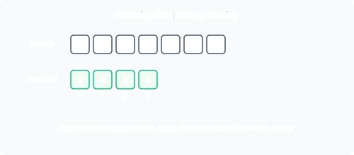
Given input array A of length $n$ and maximum value $k$:

1. Allocate a count array C[0..k], initialise all entries to 0.
2. For each element $v$ in A, increment C[v].
3. Convert C to cumulative counts: for $i = 1$ to $k$, set C[i] = C[i] + C[i-1]. Now C[i] is the number of elements $\le i$.
4. Allocate output array B[1..n]. Iterate through A from right to left (to preserve stability): for each $v = A[j]$, place it at B[C[v]], then decrement C[v].

The right-to-left pass in step 4 is what guarantees stability: when duplicate values exist, the element appearing later in the input is placed later in the output.

Worked Example

Sort A = [2, 5, 3, 0, 2, 3, 0, 3] with $k = 5$.

Step 1: Count occurrences

$i$	0	1	2	3	4	5
C[i]	2	0	2	3	0	1

Step 2: Cumulative counts

$i$	0	1	2	3	4	5
C[i]	2	2	4	7	7	8

Interpretation: there are 2 elements $\le 0$, 2 elements $\le 1$, 4 elements $\le 2$, etc. So the value 2 will occupy output positions 3 and 4 (1-indexed: C[2] = 4, then decrement yields 3 for next occurrence).

Step 3: Place elements (right to left)

• $A[8] = 3$: C[3] = 7 → B[7] = 3, C[3] = 6
• $A[7] = 0$: C[0] = 2 → B[2] = 0, C[0] = 1
• $A[6] = 3$: C[3] = 6 → B[6] = 3, C[3] = 5
• $A[5] = 2$: C[2] = 4 → B[4] = 2, C[2] = 3
• $A[4] = 0$: C[0] = 1 → B[1] = 0, C[0] = 0
• $A[3] = 3$: C[3] = 5 → B[5] = 3, C[3] = 4
• $A[2] = 5$: C[5] = 8 → B[8] = 5, C[5] = 7
• $A[1] = 2$: C[2] = 3 → B[3] = 2, C[2] = 2

Output: B = [0, 0, 2, 2, 3, 3, 3, 5]. Notice that the two 0s preserve their original relative order, as do the two 2s and three 3s. The sort is stable.

Complexity Analysis

Step	Cost
Initialise C[0..k]	$\Theta(k)$
Count occurrences	$\Theta(n)$
Cumulative counts	$\Theta(k)$
Place elements	$\Theta(n)$
Total	$\Theta(n + k)$

Space: $\Theta(n + k)$ for the output array and count array. Counting sort is not in-place.

When Is It Linear?

If $k = O(n)$, then $\Theta(n + k) = \Theta(n)$. This is the practical regime. If $k$ is much larger than $n$ (e.g. sorting a handful of 64-bit integers), then counting sort is $\Theta(k)$-dominated and wastes both time and space.

Why It Beats the Lower Bound

The $\Omega(n \log n)$ lower bound applies only to comparison-based sorting. Counting sort never compares elements against each other; it inspects the numerical value of each key directly and uses that value as an array index. This is not a valid operation in the comparison model.

Stability

Counting sort is stable because we iterate the input from right to left when placing elements. The last occurrence of a value in the original array is placed at the rightmost available position for that value in the output, preserving relative order amongst equal keys.

Summary

Property	Value
Type	Non-comparison, integer sort
Worst-case time	$\Theta(n + k)$
Space	$\Theta(n + k)$
Stable	Yes
In-place	No
Practical when	$k = O(n)$
Beats $\Omega(n \log n)$	Yes (not comparison-based)