Bucket Sort

Overview

Bucket sort distributes $n$ inputs into $k$ buckets according to their key range, sorts each bucket individually (typically with insertion sort), and concatenates the buckets in order. It assumes the input is drawn uniformly from a known interval. Under this assumption, each bucket receives approximately $n/k$ elements and the average-case running time is $\Theta(n)$.

Worst-case running time is $\Theta(n^2)$ if all elements fall into one bucket, since insertion sort on $n$ elements is $\Theta(n^2)$.

Algorithm

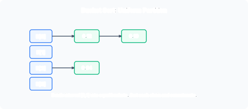
For input in the range $[0, 1)$:

1. Create $n$ empty buckets (linked lists or arrays).
2. For each element $x$, insert it into bucket $\lfloor n \cdot x \rfloor$.
3. Sort each bucket (e.g. with insertion sort).
4. Concatenate buckets in order (0, 1, …, $n-1$).

The bucket index $\lfloor n \cdot x \rfloor$ maps the uniform $[0, 1)$ range onto $n$ equal-width intervals.

Worked Example

Input: $[0.78, 0.17, 0.39, 0.26, 0.72, 0.94, 0.21, 0.12, 0.23, 0.68]$, $n = 10$.

Step 2: Distribute into buckets ($\lfloor 10 \cdot x \rfloor$):

Bucket	Range	Elements
0	$[0, 0.1)$	—
1	$[0.1, 0.2)$	0.17, 0.12
2	$[0.2, 0.3)$	0.26, 0.21, 0.23
3	$[0.3, 0.4)$	0.39
4	$[0.4, 0.5)$	—
5	$[0.5, 0.6)$	—
6	$[0.6, 0.7)$	0.68
7	$[0.7, 0.8)$	0.78, 0.72
8	$[0.8, 0.9)$	—
9	$[0.9, 1.0)$	0.94

Step 3: Sort each bucket (insertion sort):

• Bucket 1: $[0.12, 0.17]$
• Bucket 2: $[0.21, 0.23, 0.26]$
• Bucket 3: $[0.39]$
• Bucket 6: $[0.68]$
• Bucket 7: $[0.72, 0.78]$
• Bucket 9: $[0.94]$

Step 4: Concatenate: $[0.12, 0.17, 0.21, 0.23, 0.26, 0.39, 0.68, 0.72, 0.78, 0.94]$

Complexity Analysis

Distribution into $n$ buckets: $\Theta(n)$. Sorting each bucket: let $n_i$ be the number of elements in bucket $i$. Insertion sort on bucket $i$ costs $O(n_i^2)$. Total:

$T(n) = \Theta(n) + \sum_{i=0}^{n-1} O(n_i^2)$

Under the uniform distribution assumption, the expected value of $n_i^2$ is $2 - 1/n$, giving $T(n) = \Theta(n) + n \cdot O(2 - 1/n) = \Theta(n)$.

If the uniformity assumption fails and all $n$ elements land in one bucket, insertion sort on that bucket costs $\Theta(n^2)$, which is the worst case.

Comparison with Counting Sort and Radix Sort

Sort	Assumption	Average	Worst
Counting sort	Integer keys in $[0, k]$	$\Theta(n + k)$	$\Theta(n + k)$
Radix sort	$d$-digit integers	$\Theta(d(n + k))$	$\Theta(d(n + k))$
Bucket sort	Uniform real keys in $[0, 1)$	$\Theta(n)$	$\Theta(n^2)$

Bucket sort is the only one of the three whose worst case is quadratic. Its average-case speed depends on the uniform-distribution assumption, whereas counting and radix sort guarantee their bounds for all inputs satisfying their range constraints.

Practical Use

Bucket sort is most useful when input is known to be uniformly distributed — for example, hashing a uniform key space into buckets. In practice, it is often combined with other techniques (e.g. using a better sort within buckets, or using it as one phase of a hybrid algorithm).

Summary

Property	Value
Type	Non-comparison, distribution sort
Average time	$\Theta(n)$
Worst-case time	$\Theta(n^2)$
Space	$\Theta(n)$ for buckets
Stable	Depends on bucket sort
Assumption	Uniform distribution of keys
Beats $\Omega(n \log n)$	Yes on average (not comparison-based)