Skip to content
Back to Modules
Part IA Lent Term

Machine Learning and Real-World Data

Machine-Learning Classification Naive-Bayes Hidden-Markov-Models Networks Graph-Theory Clustering K-Means Ethics Bias Part IA Lent Term Paper 3
  • Methodology, Evaluation, and Significance Testing

    Train/dev/test splits, cross-validation, confusion matrices and derived metrics, the sign test, permutation tests, and Type 1/Type 2 errors

    • Train, Development, and Test Splits

      The Golden Rule

      Before performing any analysis on a dataset, partition it into three disjoint subsets: training, development (validation), and test. This separation prevents data leakage and preserves the validity of statistical evaluation.

      Training Set

      The training set is used strictly for fitting model parameters. For a Naive Bayes classifier, this means counting word-class co-occurrences and estimating priors. The model sees these examples during learning; no evaluation happens here.

      Typical proportion: 60-80% of the total data.

      Development (Validation) Set

      The development set tunes hyperparameters, selects features, and debugs the model. You may evaluate on this set repeatedly whilst iterating on the model: adjusting the smoothing parameter ω\omega, choosing which features to include, comparing different model architectures.

      Typical proportion: 10-20% of the total data.

      Test Set

      The test set is used exactly once: to report the final, unbiased performance of the chosen model. It must remain completely unseen throughout development. The model’s parameters must never be influenced by test-set performance.

      Typical proportion: 10-20% of the total data.

      The Multiple Comparisons Problem

      If you check the test set repeatedly during development (even “just to see how things are going”), you are implicitly tuning to it. Each peek constitutes a comparison; across many peeks, the model that happens to score highest on this particular test split will be selected. The test set is no longer “unseen”, and statistical significance tests become invalid.

      A common exam scenario: a student develops a model over 20 iterations, checking test-set accuracy after each change. On the final iteration, they obtain 85% and claim significance. This is wrong: the model was selected precisely because it happened to look best on that test split. The p-value associated with that 85% is meaningless, since the test data has been incorporated into the model selection process.

      Simple Diagram

      A typical data split maps as follows: 70% of the original data becomes the training set. Of the remaining 30%, half (15% of total) forms the development set and half (15% of total) forms the held-out test set. The training set fits the model; the development set guides feature and hyperparameter selection; the test set provides one final, honest evaluation number.

      Summary

      SplitPurposeTouched
      TrainingFit parameters (counts, priors)Every training run
      DevelopmentTune hyperparameters, select featuresRepeatedly during development
      TestFinal unbiased evaluationONCE only

      Past paper questions: y2021p3q9, y2023p3q8
    • Cross-Validation

      N-Fold Cross-Validation

      When data is limited, a single train-dev-test split wastes precious training examples. N-fold cross-validation (CV) maximises data usage: divide the data into NN equal folds, train on N1N-1 folds, test on the remaining fold, and rotate until every fold has served as the test set. Report the mean and variance of the metric across folds.

      For N=5N=5 and 100 documents: partition into 5 folds of 20 documents each. In each round, train on 80 documents, test on 20. After 5 rounds, average the 5 accuracy scores (or F1 scores).

      Five-fold or ten-fold CV is standard. Ten-fold gives lower bias but higher variance; five-fold is computationally cheaper.

      Stratified Cross-Validation

      Standard CV splits data randomly. With imbalanced classes (e.g., 90% OK messages, 10% bullying), a random split could place all bullying messages in one fold, distorting evaluation. Stratified CV ensures each fold preserves the overall class distribution: if the full dataset is 90/10, every fold is also ~90/10.

      Stratified CV is essential for any imbalanced classification task.

      Leave-One-Out CV (Jack-Knifing)

      The extreme case: NN equals the number of data points. For 100 documents, train on 99 and test on 1, repeating 100 times. This maximises training data and gives the least biased estimate of performance. The cost is high: 100 training runs, each on nearly the full dataset. Only practical for very small datasets (tens of items).

      Dependency-Sensitive Cross-Validation

      When data points are not independent (e.g., multiple documents by the same author, or from the same publication venue), random CV overestimates generalisation. The model memorises author style rather than learning the task.

      Dependency-sensitive CV folds by domain: all documents from author X go into a single fold, ensuring the model is tested on genuinely unseen authors, genres, or sources. This tests true out-of-domain generalisation.

      Worked Example

      A dataset contains 100 documents across 2 classes (60 OK, 40 bullying). With 5-fold stratified CV:

      • Each fold holds 20 documents: 12 OK and 8 bullying (preserving the 60/40 ratio).
      • In round 1: train on folds 2-5 (80 documents, 48 OK + 32 bullying), test on fold 1.
      • After 5 rounds: compute mean accuracy = 0.87, variance = 0.002.
      • Report: “87% accuracy (SD = 4.5%) across 5-fold stratified CV.”

      Without stratification, a fold might contain only 2 bullying messages, producing unreliable per-fold estimates and inflating variance.

      Summary

      MethodHow it worksWhen to use
      N-fold CVTrain on N-1 folds, test on 1, rotateLimited data, standard approach
      Stratified CVPreserve class distribution per foldImbalanced data
      Leave-one-outN = dataset sizeTiny datasets; computationally expensive
      Dependency-sensitive CVFold by domain (author, source, genre)Testing generalisation to new domains

      Past paper questions: y2021p3q9 (evaluation strategy)

    • The Confusion Matrix and Evaluation Metrics

      The 2×2 Confusion Matrix

      The 2x2 confusion matrix showing TP, FP, FN, TN cells with evaluation formulae

      For binary classification, every prediction falls into one of four cells:

      Truth: PositiveTruth: Negative
      System says: PositiveTP (True Positive)FP (False Positive)
      System says: NegativeFN (False Negative)TN (True Negative)
      • TP: correctly identified positives (bullies caught)
      • FP: false alarms (innocent messages flagged)
      • FN: missed positives (bullies that slipped through)
      • TN: correctly identified negatives (innocent messages passed)

      Accuracy

      Accuracy=TP+TNTP+FP+FN+TN\text{Accuracy} = \frac{\text{TP} + \text{TN}}{\text{TP} + \text{FP} + \text{FN} + \text{TN}}

      Accuracy is misleading when classes are imbalanced. A classifier that labels every message “OK” on a dataset with 95% OK messages achieves 95% accuracy, yet detects zero bullying. Always check class distribution before trusting accuracy.

      Precision

      Precision=TPTP+FP\text{Precision} = \frac{\text{TP}}{\text{TP} + \text{FP}}

      Of all messages the system claimed were bullying, what fraction truly were? High precision means when the system flags something, you can trust it.

      Prioritise high precision when: medical treatment decisions, legal evidence flagging, any domain where false alarms carry high cost.

      Recall

      Recall=TPTP+FN\text{Recall} = \frac{\text{TP}}{\text{TP} + \text{FN}}

      Of all actual bullying messages, what fraction did the system find? High recall means few bullies are missed.

      Prioritise high recall when: disease screening, spam detection, brand-attack detection, any domain where missing a positive is worse than a false alarm.

      F1 Score

      F1=2×Precision×RecallPrecision+Recall\text{F1} = 2 \times \frac{\text{Precision} \times \text{Recall}}{\text{Precision} + \text{Recall}}

      The harmonic mean of precision and recall. F1 penalises extreme imbalance: if precision = 0.9 and recall = 0.1, F1 = 0.18 (not 0.5). This makes F1 more honest than the arithmetic mean.

      Prioritise high F1 when: most NLP classification tasks, balanced trade-off needed.

      Worked Example

      A bullying-filter classifier is evaluated on 1000 messages, of which 100 are truly bullying:

      Truth: BullyingTruth: OK
      System says: BullyingTP = 80FP = 40
      System says: OKFN = 20TN = 860
      • Accuracy = (80 + 860) / 1000 = 0.94 (94%)
      • Precision = 80 / (80 + 40) = 80/120 = 0.667
      • Recall = 80 / (80 + 20) = 80/100 = 0.80
      • F1 = 2 × (0.667 × 0.80) / (0.667 + 0.80) = 2 × 0.534 / 1.467 = 0.728

      Accuracy looks excellent at 94%, but that is driven by the 860 TNs. Precision and recall reveal that one third of flagged messages are false alarms, and one fifth of bullies are missed.

      Note: precision and recall are always defined with respect to a specific class (here, bullying). There is no such thing as “overall precision” without specifying the class of interest.

      Summary

      MetricFormulaUse
      Accuracy(TP+TN)/TotalBalanced classes only
      PrecisionTP/(TP+FP)When false alarms are costly
      RecallTP/(TP+FN)When missing positives is costly
      F12PR/(P+R)Balanced trade-off

      Past paper questions: y2021p3q9(b)

    • Macro vs Micro Averaging for Multi-Class Problems

      Why Averaging Matters

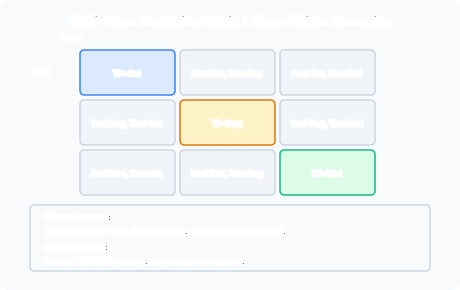
      3-class confusion matrix showing how macro and micro averaging differ in their aggregation

      With more than two classes, a single precision/recall/F1 number per class tells only part of the story. We need a way to aggregate per-class metrics into one overall score. The choice between macro and micro averaging determines which classes drive the final number.

      Macro-Averaging

      Compute the metric (e.g., F1) for each class independently, then take the arithmetic mean across classes. Every class contributes equally, regardless of how many examples it has.

      Macro-F1=1CcCF1c\text{Macro-F1} = \frac{1}{|C|} \sum_{c \in C} \text{F1}_c

      Best for imbalanced data where minority classes matter. If class A has 1000 examples and class B has 10, macro-F1 gives them equal weight. A poor F1 on the minority class will noticeably drag down the macro average.

      Micro-Averaging

      Pool all TP, FP, and FN counts across classes into global totals, then compute the metric on those pooled counts.

      Micro-F1=2×cTPc2×cTPc+cFPc+cFNc\text{Micro-F1} = \frac{2 \times \sum_c \text{TP}_c}{2 \times \sum_c \text{TP}_c + \sum_c \text{FP}_c + \sum_c \text{FN}_c}

      This is equivalent to computing accuracy (when each example has exactly one label). Large classes dominate; a minority class with poor performance barely affects the score.

      Worked Example

      Consider a 3-class problem with the following per-class counts:

      ClassTPFPFNExamples
      Hardware90510100
      Theory801020100
      Ethics551520

      Per-class F1:

      • Hardware: Precision = 90/95 = 0.947, Recall = 90/100 = 0.90, F1 = 2×0.947×0.90/(0.947+0.90) = 0.923
      • Theory: Precision = 80/90 = 0.889, Recall = 80/100 = 0.80, F1 = 0.842
      • Ethics: Precision = 5/10 = 0.50, Recall = 5/20 = 0.25, F1 = 0.333

      Macro-F1 = (0.923 + 0.842 + 0.333) / 3 = 0.699

      Micro-F1: pool all counts.

      Total TP = 90 + 80 + 5 = 175 Total FP = 5 + 10 + 5 = 20 Total FN = 10 + 20 + 15 = 45

      Micro-Precision = 175/(175+20) = 0.897 Micro-Recall = 175/(175+45) = 0.795 Micro-F1 = 2×0.897×0.795/(0.897+0.795) = 0.844

      The macro-F1 (0.699) reflects the poor Ethics performance. The micro-F1 (0.844) is dominated by the two large classes and hides the Ethics problem. When minority classes matter, report macro-averaged metrics; when overall throughput matters, micro-averaging suffices.

      Summary

      AveragingHowWeightBest for
      MacroPer-class metric then averageEqual per classImbalanced data, minority classes matter
      MicroPool all TP/FP/FN then computeProportional to class sizeOverall throughput, balanced classes

      Past paper questions: y2023p3q8(b) (per-area evaluation)

    • The Multiple Comparisons Problem

      The Problem

      Repeatedly evaluating on the test set during development makes the test set no longer “unseen”. Each evaluation is a comparison; across many comparisons, the model that happens to look best on this particular random split is selected. Statistical significance tests assume a single, pre-planned comparison against fresh data. Using the same test set across iterations violates this assumption.

      Why p-Values Break

      A p-value of 0.03 means: “if the null hypothesis were true, there is a 3% chance of observing a result this extreme.” This relies on the test data being a single fresh draw. If you have tested 50 model variants on the same test set, you have effectively run 50 comparisons. The probability that at least one variant looks “significant” at α=0.05\alpha = 0.05 purely by chance is:

      P(at least one significant)=1(10.05)500.923P(\text{at least one significant}) = 1 - (1 - 0.05)^{50} \approx 0.923

      There is a 92% chance that pure noise will produce at least one “significant” result. The p-value of the winning variant is meaningless, because that variant won precisely because it overfit the noise in the test set.

      Common Exam Scenario

      A student splits data into train/test, then develops a classifier over 15 iterations:

      1. Train on training set
      2. Evaluate on test set
      3. Adjust features based on test-set performance
      4. Repeat

      On iteration 15, accuracy = 88%. The student computes a p-value and claims the classifier is significantly better than a baseline. This is invalid. The model was selected from 15 candidates based on test-set performance. The test set has been incorporated into the model selection process. The 88% is optimistically biased, and the associated p-value is incorrect.

      The Correct Approach

      Split data into three portions: train, dev, test. Use the dev set for all iterative development (feature selection, hyperparameter tuning, model selection). Only when the final model is locked down, evaluate once on the test set and report that single number as the honest performance estimate. The test set is touched exactly once.

      Connection to the Sign Test

      The same logic applies to significance testing between systems. If you run a sign test on the test set, then tweak the system and run another sign test on the same test set, you are performing multiple comparisons. The second test’s p-value is invalid unless corrected. The test set must be held out from all development and only used for one pre-planned significance test.

      Summary

      IssueCauseConsequence
      Multiple comparisonsRepeated test-set evaluation during developmentp-values become invalid
      Optimistic biasSelecting model that looks best on test splitReported performance is inflated
      Correct fixUse separate dev set for iteration; test set onceValid statistical inference

      Past paper questions: y2021p3q9 (evaluation strategy)

    • The Sign Test

      Purpose

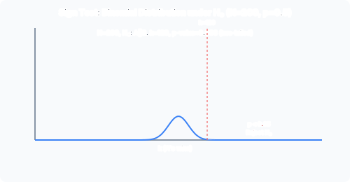
      Binomial distribution under H0 showing critical region at k=120 for N=200 with p<0.05

      The sign test determines whether System A is significantly better than System B on a classification task. It tests the null hypothesis that both systems are equally good and any observed differences are due to chance.

      Setup

      • H0 (null hypothesis): Systems A and B are identical; differences are due to chance.
      • H1 (alternative): System A is better than System B (one-tailed) or systems differ (two-tailed).
      • Compare item by item: for each document, note whether A wins, B wins, or they tie.

      The MLRD Tie Rule (CRITICAL)

      Standard statistics textbooks say to discard ties. For classification tasks, this is wrong. Discarding ties reduces NN, inflating the test statistic and causing a Type 1 error (falsely claiming significance).

      The MLRD rule: distribute ties evenly. Let dd = number of ties. Add d/2d/2 to kk (A’s wins) and d/2d/2 to (Nk)(N - k) (B’s wins). Round kk up at the end. NN remains unchanged.

      Test Statistic

      Under H0, each item is equally likely to favour A or B (ignoring ties). Test statistic:

      XBinomial(N,p=0.5)X \sim \text{Binomial}(N, p = 0.5)

      k=items where A beats B+d2k = \text{items where A beats B} + \frac{d}{2}

      • One-tailed p-value: P(XkN,p=0.5)P(X \geq k \mid N, p=0.5)
      • Two-tailed p-value: 2×P(XkN,p=0.5)2 \times P(X \geq k \mid N, p=0.5)

      If p0.05p \leq 0.05: reject H0; A is significantly better. If p>0.05p > 0.05: inconclusive; cannot claim A is better.

      Full Worked Example

      200 documents are classified by both System A and System B:

      • A wins on 110 documents
      • B wins on 70 documents
      • Ties on 20 documents

      Step 1 — Apply the tie rule: k=110+20/2=110+10=120k = 110 + 20/2 = 110 + 10 = 120 N=200N = 200 (unchanged) (Nk)=200120=80(N - k) = 200 - 120 = 80

      Step 2 — Two-tailed test: We test whether A differs from B (in either direction). Under H0, XBinomial(200,0.5)X \sim \text{Binomial}(200, 0.5).

      p=2×P(X120N=200,p=0.5)p = 2 \times P(X \geq 120 \mid N=200, p=0.5)

      For a binomial with N=200N=200, p=0.5p=0.5, the mean is Np=100Np = 100 and variance is Np(1p)=50Np(1-p) = 50. We can approximate using the normal distribution:

      z=kNpNp(1p)=12010050=207.0712.828z = \frac{k - Np}{\sqrt{Np(1-p)}} = \frac{120 - 100}{\sqrt{50}} = \frac{20}{7.071} \approx 2.828

      From standard normal tables: P(Z2.828)0.0023P(Z \geq 2.828) \approx 0.0023.

      Two-tailed p=2×0.0023=0.0046p = 2 \times 0.0023 = 0.0046.

      Step 3 — Conclusion: p=0.0046<0.05p = 0.0046 < 0.05. Reject H0. System A is significantly better than System B.

      If we had discarded ties (wrong): N=180N = 180, k=110k = 110, z=(11090)/45=20/6.7082.981z = (110 - 90)/\sqrt{45} = 20/6.708 \approx 2.981, giving a smaller p-value. This inflates the apparent significance, risking a false claim.

      Why Not Discard Ties?

      Discarding ties reduces NN from 200 to 180. The test statistic z=(kN/2)/N/4z = (k - N/2)/\sqrt{N/4} increases because the denominator N\sqrt{N} shrinks while the numerator stays similar. This makes the test more likely to reject H0 even when A and B are truly identical (Type 1 error). The MLRD rule keeps NN fixed and distributes ties as half-wins, which is more conservative and honest.

      Summary

      StepAction
      1Count A wins, B wins, ties
      2k=A wins+(ties/2)k = \text{A wins} + (\text{ties}/2), round up
      3NN unchanged
      4Compute p=P(XkBinomial(N,0.5))p = P(X \geq k \mid \text{Binomial}(N, 0.5))
      5If two-tailed, multiply by 2
      6Compare to α=0.05\alpha = 0.05

      Past paper questions: y2023p3q8 (evaluation methods)

    • The Permutation Test

      Purpose

      The permutation test (also called the randomisation test) is a more powerful alternative to the sign test for determining whether System A is significantly better than System B. It naturally handles ties without the MLRD special tie rule, because it operates on the actual metric values rather than win/loss/tie counts.

      Intuition

      Under H0, both systems are equally good: their predictions for any given document are interchangeable. If we randomly swap the predictions of A and B for some documents, the overall performance difference should not systematically change. If the observed difference is larger than what we would see under random swapping, we have evidence that A is genuinely better.

      Procedure

      1. Compute observed difference: Δobs=metric(A)metric(B)\Delta_{\text{obs}} = \text{metric}(A) - \text{metric}(B), e.g., the difference in F1 scores.

      2. Enumerate permutations: There are 2N2^N possible ways to swap predictions between A and B (for each of NN documents, either swap or do not swap).

      3. For each permutation: apply the swaps, recompute Δperm\Delta_{\text{perm}}, and record the result.

      4. Compute p-value: the proportion of permutations where ΔpermΔobs\vert \Delta_{\text{perm}} \rvert \geq \vert \Delta_{\text{obs}} \rvert (two-tailed) or ΔpermΔobs\Delta_{\text{perm}} \geq \Delta_{\text{obs}} (one-tailed).

      5. Decision: if p0.05p \leq 0.05, reject H0.

      Monte Carlo Approximation

      For N=100N = 100 documents, 21002^{100} permutations is impossible to enumerate. In practice, we use a Monte Carlo permutation test: randomly sample a large number of permutations (e.g., 10,000) rather than exhaustively enumerating all. The p-value is the proportion of sampled permutations where the difference meets or exceeds the observed one.

      Why More Powerful Than the Sign Test

      The sign test reduces each document to a ternary outcome (A wins, B wins, tie) and discards the magnitude of the difference. If A beats B by a tiny margin on 60 documents and loses by a huge margin on 40, the sign test treats the 60 as “wins” and the 40 as “losses”, potentially missing the fact that B’s victories are much larger.

      The permutation test uses the actual metric values. It captures both the direction and the magnitude of each difference. Ties are naturally absorbed into the metric, since identical predictions produce a difference of zero.

      Worked Example

      Suppose we have 10 documents. System A achieves F1 = 0.82; System B achieves F1 = 0.74. The observed difference: Δobs=0.08\Delta_{\text{obs}} = 0.08.

      Under H0, each document’s pair of predictions (A’s label, B’s label) can be swapped or left as-is. We generate 1,000 random permutations. In each, we randomly swap the predictions for a random subset of documents, recompute F1 for both systems, and compute Δperm\Delta_{\text{perm}}.

      Suppose 23 out of 1,000 permutations produce Δperm0.08\vert \Delta_{\text{perm}} \rvert \geq 0.08.

      p=23/1000=0.023p = 23/1000 = 0.023

      Since 0.023<0.050.023 < 0.05, reject H0. System A’s improvement is statistically significant.

      Summary

      AspectSign TestPermutation Test
      InputWin/loss/tie per itemMetric value (e.g., F1, accuracy)
      Tie handlingSpecial MLRD rule requiredNatural; ties produce zero difference
      PowerLower (discards magnitude)Higher (uses actual values)
      ComputationLightweight2N2^N or Monte Carlo sampling

      Past paper questions: y2023p3q8 (evaluation)

    • Type 1 and Type 2 Errors, Power, and Specificity

      The Four Outcomes

      Every significance test yields one of four outcomes, depending on the true state of the world and the test’s conclusion:

      H0 is TRUEH0 is FALSE
      Reject H0Type 1 Error (α\alpha)Correct rejection (Power, 1β1-\beta)
      Do NOT reject H0Correct non-rejection (Specificity, 1α1-\alpha)Type 2 Error (β\beta)

      Type 1 Error (False Positive, α\alpha)

      Rejecting H0 when it is actually true: claiming System A is better when it is not. The significance level α=0.05\alpha = 0.05 means we accept a 5% chance of committing a Type 1 error every time we run a test.

      If we run 20 independent tests at α=0.05\alpha = 0.05, the expected number of Type 1 errors is 1. This is the multiple comparisons problem: across many tests, some will appear significant purely by chance.

      Type 2 Error (False Negative, β\beta)

      Failing to reject H0 when it is actually false: missing a real improvement. β\beta is the probability of a Type 2 error. Unlike α\alpha (which we set explicitly), β\beta depends on the true effect size, sample size, and test power. A small sample makes β\beta large: real differences go undetected.

      Power (1β1 - \beta)

      The probability of correctly rejecting a false H0: detecting a real difference when one exists. Higher power is better. Power increases with:

      • Larger sample size NN
      • Larger true effect size
      • More sensitive test (permutation test is more powerful than sign test)

      A test with low power cannot reliably detect real improvements. If you fail to reject H0 with a small dataset, you cannot conclude “A and B are the same”; you can only conclude “the data are insufficient to tell.”

      Specificity (1α1 - \alpha)

      The probability of correctly not rejecting a true H0: guarding against false discoveries. If α=0.05\alpha = 0.05, specificity = 0.95. Raising the significance threshold (e.g., α=0.01\alpha = 0.01) increases specificity but reduces power.

      The Trade-Off

      α\alpha and β\beta are in tension. Lowering α\alpha (making it harder to reject H0) reduces Type 1 errors but increases Type 2 errors (since you need stronger evidence to reject). Raising α\alpha increases power but also increases false positives.

      The standard α=0.05\alpha = 0.05 balances Type 1 and Type 2 errors for most applications. In safety-critical domains (medical treatment), a lower α\alpha (more conservative) may be warranted to avoid false positives. In exploratory research, a higher α\alpha may be acceptable to avoid missing genuine signals.

      Worked Example

      A sign test on 200 documents compares two spam filters. H0: filters are equally good. The observed test statistic gives p=0.03p = 0.03. We reject H0 at α=0.05\alpha = 0.05 and conclude Filter A is significantly better.

      If H0 were actually true (filters are identical), we have committed a Type 1 error: the significant result was a fluke. There is a 5% chance of this occurring, and it did.

      If H0 were actually false (Filter A is genuinely better) and we had instead obtained p=0.07p = 0.07, we would fail to reject H0: a Type 2 error. The test lacked power to detect a real difference.

      Summary

      ConceptSymbolMeaning
      Type 1 Errorα\alphaFalse positive: claiming A is better when it is not
      Type 2 Errorβ\betaFalse negative: missing a real improvement
      Power1β1-\betaCorrectly detecting a real improvement
      Specificity1α1-\alphaCorrectly avoiding false discoveries

      Past paper questions: y2023p3q8 (evaluation)

  • Inter-Annotator Agreement

    Cohen's Kappa for two annotators, Fleiss' Kappa for multiple annotators, handling partial annotation, and crowdsourcing pitfalls

    • Cohen's Kappa for Two Annotators

      Why Raw Agreement Misleads

      If two annotators label items independently, simply counting how often they agree gives a misleading picture. Even if both annotators guess randomly, they will agree by chance some fraction of the time. With few classes (e.g., binary labels), chance agreement can be high: two annotators both guessing “OK” 50% of the time agree by chance 50% of the time.

      Cohen’s κ\kappa corrects for this: it measures agreement above chance, normalised by the maximum possible agreement above chance.

      Formula

      κ=P(A)P(E)1P(E)\kappa = \frac{P(A) - P(E)}{1 - P(E)}

      • P(A)P(A): observed agreement — proportion of items where both annotators gave the same label.
      • P(E)P(E): expected chance agreement — the probability they would agree if both guessed independently based on their observed label distributions.

      P(E)=cClassesP(Ann1 chooses c)×P(Ann2 chooses c)P(E) = \sum_{c \in \text{Classes}} P(\text{Ann}_1 \text{ chooses } c) \times P(\text{Ann}_2 \text{ chooses } c)

      Interpretation

      • κ=1.0\kappa = 1.0: perfect agreement
      • κ>0.8\kappa > 0.8: strong agreement
      • κ>0.6\kappa > 0.6: acceptable agreement
      • κ=0.0\kappa = 0.0: no better than chance
      • κ<0\kappa < 0: worse than chance (systematic disagreement)

      Full Worked Example (2023 Q7)

      Two annotators (A and B) classify 8 items into 4 classes (I, II, III, IV). Data:

      Item12345678
      AIIIIVIIIIIIIVII
      BIIIIIIIVIVIIVI

      Step 1 — Observed agreement P(A)P(A): Items where A = B: item 1 (III=III), item 3 (II=II), item 6 (I=I), item 7 (IV=IV).

      P(A)=4/8=0.5P(A) = 4/8 = 0.5

      Step 2 — Marginal frequencies for A:

      • PA(I)=2/8=0.25P_A(\text{I}) = 2/8 = 0.25
      • PA(II)=3/8=0.375P_A(\text{II}) = 3/8 = 0.375
      • PA(III)=1/8=0.125P_A(\text{III}) = 1/8 = 0.125
      • PA(IV)=2/8=0.25P_A(\text{IV}) = 2/8 = 0.25

      Step 3 — Marginal frequencies for B:

      • PB(I)=3/8=0.375P_B(\text{I}) = 3/8 = 0.375
      • PB(II)=1/8=0.125P_B(\text{II}) = 1/8 = 0.125
      • PB(III)=1/8=0.125P_B(\text{III}) = 1/8 = 0.125
      • PB(IV)=3/8=0.375P_B(\text{IV}) = 3/8 = 0.375

      Step 4 — Expected chance agreement P(E)P(E):

      P(E)=(0.25×0.375)+(0.375×0.125)+(0.125×0.125)+(0.25×0.375)P(E) = (0.25 \times 0.375) + (0.375 \times 0.125) + (0.125 \times 0.125) + (0.25 \times 0.375)

      P(E)=0.09375+0.046875+0.015625+0.09375=0.25P(E) = 0.09375 + 0.046875 + 0.015625 + 0.09375 = 0.25

      Step 5 — Compute κ\kappa:

      κ=0.50.2510.25=0.250.75=0.333\kappa = \frac{0.5 - 0.25}{1 - 0.25} = \frac{0.25}{0.75} = 0.333

      Interpretation: moderate agreement, well above chance (κ=0.0\kappa = 0.0) but far from strong (κ>0.8\kappa > 0.8). The annotators do better than random guessing but disagree substantially.

      Why This Matters for ML

      If human annotators achieve only κ=0.333\kappa = 0.333 on a task, a classifier trained on their labels cannot realistically exceed that performance. The inter-annotator agreement sets an upper bound on achievable classifier accuracy. Low κ\kappa indicates the task itself is subjective, and the “ground truth” labels are noisy.

      Summary

      ComponentMeaningThis example
      P(A)P(A)Observed agreement0.5 (4 of 8)
      P(E)P(E)Chance agreement0.25
      κ\kappaAgreement above chance, normalised0.333

      Past paper questions: y2023p3q7(b), y2021p3q9(c)

    • Fleiss' Kappa for Multiple Annotators

      When Cohen’s Kappa Is Not Enough

      Cohen’s κ\kappa works for exactly two annotators. When you have three or more annotators (e.g., a crowd of workers each labelling items), you need Fleiss’ κ\kappa, which generalises the chance-corrected agreement measure to an arbitrary number of raters.

      Notation

      • NN: number of items
      • kk: number of annotators per item (can vary per item in the generalised version)
      • CC: number of categories (classes)
      • nijn_{ij}: number of annotators who assigned category jj to item ii

      Formula

      Observed agreement per item:

      Pa,i=j=1Cnij(nij1)k(k1)P_{a,i} = \frac{\sum_{j=1}^{C} n_{ij}(n_{ij} - 1)}{k(k - 1)}

      The numerator counts agreeing pairs for item ii (summed over categories). The denominator is the total number of annotator pairs for that item. The factor of 2 in the combination formula cancels between numerator and denominator.

      Overall observed agreement:

      Pa=1Ni=1NPa,iP_a = \frac{1}{N} \sum_{i=1}^{N} P_{a,i}

      Expected chance agreement:

      For each category jj, compute the overall proportion of all annotations assigned to that class:

      pj=i=1NnijN×kp_j = \frac{\sum_{i=1}^{N} n_{ij}}{N \times k}

      Then:

      Pe=j=1Cpj2P_e = \sum_{j=1}^{C} p_j^2

      Fleiss’ κ\kappa:

      κ=PaPe1Pe\kappa = \frac{P_a - P_e}{1 - P_e}

      Interpretation follows the same scale as Cohen’s κ\kappa.

      Full Worked Example

      Three annotators (A, B, C) label 3 items as POS or NEG:

      ItemAnnotator AAnnotator BAnnotator C
      1POSPOSNEG
      2POSNEGNEG
      3POSPOSPOS

      Here N=3N=3, k=3k=3, C=2C=2.

      Step 1 — nijn_{ij} counts:

      ItemnPOSn_{\text{POS}}nNEGn_{\text{NEG}}
      121
      212
      330

      Step 2 — Pa,iP_{a,i} per item:

      Item 1: Pa,1=[2(21)+1(11)]/[3(31)]=[2+0]/6=0.333P_{a,1} = [2(2-1) + 1(1-1)] / [3(3-1)] = [2 + 0] / 6 = 0.333

      Item 2: Pa,2=[1(11)+2(21)]/6=[0+2]/6=0.333P_{a,2} = [1(1-1) + 2(2-1)] / 6 = [0 + 2] / 6 = 0.333

      Item 3: Pa,3=[3(31)+0(01)]/6=[6+0]/6=1.0P_{a,3} = [3(3-1) + 0(0-1)] / 6 = [6 + 0] / 6 = 1.0

      Step 3 — Overall PaP_a:

      Pa=(0.333+0.333+1.0)/3=1.667/3=0.556P_a = (0.333 + 0.333 + 1.0) / 3 = 1.667 / 3 = 0.556

      Step 4 — Category proportions pjp_j:

      Total annotations = 3×3=93 \times 3 = 9. POS annotations = 2+1+3=62 + 1 + 3 = 6, so pPOS=6/9=0.667p_{\text{POS}} = 6/9 = 0.667. NEG annotations = 1+2+0=31 + 2 + 0 = 3, so pNEG=3/9=0.333p_{\text{NEG}} = 3/9 = 0.333.

      Step 5 — Expected chance agreement PeP_e:

      Pe=0.6672+0.3332=0.444+0.111=0.556P_e = 0.667^2 + 0.333^2 = 0.444 + 0.111 = 0.556

      Step 6 — Fleiss’ κ\kappa:

      κ=0.5560.55610.556=00.444=0.0\kappa = \frac{0.556 - 0.556}{1 - 0.556} = \frac{0}{0.444} = 0.0

      Interpretation: agreement is no better than chance. Despite Pa=0.556P_a = 0.556 looking modestly above 50%, the chance correction reveals that the observed agreement is exactly what random guessing with the observed label proportions would produce.

      Summary

      ComponentMeaningThis example
      PaP_aMean pairwise agreement per item0.556
      PeP_eChance agreement from marginal proportions0.556
      κ\kappaFleiss’ kappa0.0 (chance-level)

      Past paper questions: y2023p3q7(b), y2021p3q9(c)

    • Handling Partial Annotation

      The Problem

      In real annotation projects, annotators often cover different subsets of items. For example, Annotator D labels items 3-8 whilst Annotator E labels items 1-8. A naive approach is to merge D and E into one “fake” annotator and treat the combined labels as if from a single rater. This creates several problems.

      Why Merging D and E Is Wrong

      1. Different conditions. D’s decisions on items 3-8 were made at a different time and possibly under different instructions or conditions than E’s decisions on items 1-8. Merging conflates these.

      2. Arbitrary bias from discarding. For items both annotated (3-8), you would need to throw away one annotation to avoid duplication. The choice of which to discard introduces arbitrary bias into the dataset.

      3. Inconsistent coverage. The “merged” annotator has an inconsistent coverage pattern: some items have one label, some have two. This makes comparisons across items unfair.

      4. Asymmetric weighting. If D covered more items than E, the “merged” annotator’s label distribution is skewed toward D’s tendencies. The merged pseudo-annotator is not a real rater; it is a statistical artefact.

      The Correct Approach

      Adapt Fleiss’ κ\kappa (or Cohen’s κ\kappa) to handle variable annotator coverage:

      1. Calculate PaP_a only over overlapping items. An item contributes to PaP_a only if it was labelled by at least two of the full annotator set. For items labelled by only one annotator, no agreement can be computed; they are excluded from the numerator.

      2. Calculate PeP_e from all available annotations. The marginal proportions pjp_j (how often each class is chosen) are computed across the full dataset, including items with only one label. This gives unbiased estimates of each class’s overall frequency.

      3. Use per-item kk. The denominator k(k1)k(k-1) for each item uses the number of annotators who actually labelled that specific item, not a global kk. An item labelled by 2 annotators uses 2×1=22 \times 1 = 2; an item labelled by 5 annotators uses 5×4=205 \times 4 = 20.

      Example

      Consider a dataset with 5 annotators {A, B, C, D, E} and 8 items. A, B, and C label all 8 items. D labels items 3-8. E labels items 1-8.

      For computing PaP_a:

      • Items 3-8 are labelled by all 5 annotators: PaP_a uses these 6 items with k=5k=5.
      • Items 1-2 are labelled by A, B, C, E: PaP_a uses these 2 items with k=4k=4.

      For computing PeP_e:

      • All 8 items contribute to the marginal proportions pjp_j.
      • Total annotations = (3×8)+6+8=38(3 \times 8) + 6 + 8 = 38 (not 5×8=405 \times 8 = 40).

      The global PaP_a is the mean of per-item Pa,iP_{a,i} values across all items that have at least 2 annotators.

      Why This Matters

      Partial annotation is the norm in practical projects. Crowd workers drop out, annotators have different availability, and budgets constrain coverage. Using the correct per-item kk and overlapping-only PaP_a prevents inflated or deflated agreement estimates that would misrepresent annotation quality.

      Summary

      ProblemCorrect solution
      Merging annotators conflates different conditionsKeep annotators separate; adapt the formula
      Items with single labels have no agreementExclude from PaP_a, include in PeP_e
      Variable annotator count per itemUse per-item kk in the denominator

      Past paper questions: y2023p3q7(c)

    • Crowdsourcing Problems and Pitfalls

      Why Crowdsourcing Annotations Is Difficult

      Crowdsourcing platforms distribute annotation tasks to many workers, each labelling a small batch of items. Whilst this is cheap and fast, it introduces several problems that make standard inter-annotator agreement metrics unreliable or impossible to compute.

      Problem 1: Very Small Batches

      When each worker annotates only 2-3 items, the variance in per-worker agreement estimates is enormous. A worker who happens to get two easy items looks excellent; a worker who gets two ambiguous items looks terrible. Neither estimate is reliable. With large batches (20+ items per worker), you can form stable per-worker quality estimates; with 2 items, you cannot.

      Problem 2: Random Assignment Breaks Pairwise Kappa

      Crowd workers are typically assigned random subsets of items. With hundreds of workers each labelling a few items, many annotator pairs never share a single item. Cohen’s κ\kappa requires pairs to have at least some overlapping items. Pairwise agreement between workers who never labelled the same thing cannot be computed.

      Fleiss’ κ\kappa partially solves this (it pools all annotators), but still assumes most items have multiple labels, which may not hold if workers are spread thinly.

      Problem 3: Variable Worker Quality

      Crowd workers vary widely in skill and motivation. Some are diligent experts; others spam randomly to maximise payment per unit time. A worker who labels everything “POS” will agree with other workers purely by chance on balanced datasets. Simple agreement metrics cannot distinguish genuine skill from lucky guessing or systematic spamming.

      Solutions: include gold-standard items (with known labels) to filter low-quality workers; use worker-specific quality weights in the agreement calculation; reject workers whose accuracy on gold items falls below a threshold.

      Problem 4: No Inter-Section Consistency Check

      Large annotation projects often divide items into sections, with different worker pools per section. If no workers label items across sections, there is no way to check whether labelling standards are consistent between sections. Section A’s annotators might interpret the guidelines differently from Section B’s. The resulting dataset has systematic bias between sections, but no agreement metric will reveal it because there is no overlap to measure against.

      Solution: allocate a shared subset of items across all sections. These overlap items serve as a consistency check, allowing computation of agreement between sections.

      Summary

      ProblemCauseConsequence
      Small batches2 items per workerHigh variance, unreliable quality estimates
      Random assignmentNo shared items between pairsPairwise κ\kappa impossible
      Variable qualitySome workers spam randomlyRaw agreement inflates with lucky guesses
      No inter-section overlapSections use separate worker poolsHidden systematic bias between sections

      Past paper questions: y2023p3q7(c)(ii-iii)

  • Statistical Classification

    Tokens and types, Zipf's Law and Heaps' Law, Naive Bayes classification with Laplace smoothing, log-probability underflow, and feature engineering

    • Tokens, Types, and Lexicon-Based Classification

      Tokens vs Types

      Given the sentence “The cat sat on the mat.”:

      • Token: each occurrence of a word. There are 6 tokens: “The”, “cat”, “sat”, “on”, “the”, “mat”. Count includes repetitions.
      • Type: each unique word in the vocabulary. There are 5 types: {“the”, “cat”, “sat”, “on”, “mat”}. “The” and “the” are the same type after lowercasing.

      Token count NN = total words in corpus. Type count V\lvert V \rvert = vocabulary size.

      Lexicon-Based Classification

      A lexicon is a dictionary mapping words to polarities. A simple sentiment lexicon:

      WordPolarity
      good+1
      great+2
      terrible-2
      awful-3

      To classify a document: sum the polarities of all lexicon words found. If the sum is positive, classify as positive; negative sum means negative; zero means neutral.

      Weaknesses

      1. Ignores context. “This film is not good” sums to +1 (from “good”), classified as positive. The negation is missed entirely, because the lexicon contains only unigrams.

      2. Cannot handle unseen words. If the document contains “This film is abysmal” and “abysmal” is not in the lexicon, it contributes zero. The document is classified as neutral, missing clear negative sentiment.

      3. Fixed vocabulary. Domain shifts break lexicon approaches. A general sentiment lexicon may not capture domain-specific language (e.g., “sick” in gaming communities means “impressive”, not “ill”).

      4. No weighting by importance. All lexicon words contribute equally regardless of their discriminating power. “Good” is a weak signal; “masterpiece” is strong. A lexicon with magnitudes (+1, +2, -1, -2) partially addresses this but requires manual calibration.

      Lexicon vs Naive Bayes

      Lexicon-based classification works when:

      • Very little labelled training data is available
      • Explicit, inspectable rules are needed
      • The domain is well covered by existing lexicons

      Naive Bayes works when:

      • Sufficient labelled training data exists
      • Statistical patterns capture subtle distinctions
      • Domain language differs from standard lexicons

      The two can be combined: replace words with generic <POSITIVE_WORD> / <NEGATIVE_WORD> tokens before training Naive Bayes. This bridges the lexicon’s generalisation with the classifier’s ability to learn from data.

      Summary

      ConceptDefinitionExample
      TokenEach word occurrence”the cat the cat” = 4 tokens
      TypeEach unique word”the cat the cat” = 2 types
      Lexicon-based classificationSum word polaritiesFast, interpretable, context-blind
      Lexicon + NB combinationReplace words with polarity tokensGeneralises across synonyms

      Past paper questions: y2021p3q9(e)(ii-iii), y2025p3q7(a)

    • Zipf's Law

      The Law

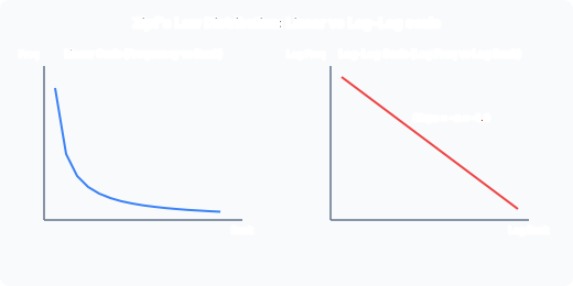
      Zipf's Law: word frequency vs rank on both linear and log-log scales showing slope -alpha

      Word frequency is inversely proportional to frequency rank. A small number of words are very frequent; a huge number of words are rare.

      Basic form:

      fw1rwf_w \propto \frac{1}{r_w}

      where fwf_w is the frequency of word ww and rwr_w is its rank (1 = most frequent).

      General form:

      fwk(rw+β)αf_w \approx \frac{k}{(r_w + \beta)^\alpha}

      • fwf_w: frequency of word ww in the corpus
      • rwr_w: frequency rank (1 = most frequent)
      • α\alpha: exponent (~1.0 for English, ~1.3 for German)
      • kk, β\beta: language-specific constants

      Log-Log Estimation

      Taking logs of the basic form:

      log(fw)=log(k)αlog(rw)\log(f_w) = \log(k) - \alpha \cdot \log(r_w)

      Plotting log(frequency)\log(\text{frequency}) against log(rank)\log(\text{rank}) gives a straight line:

      • Slope = α-\alpha (estimate α\alpha from the slope)
      • Y-intercept = log(k)\log(k) (estimate k=einterceptk = e^{\text{intercept}})

      Estimate α\alpha and kk by fitting a least-squares regression to the log-log plot.

      The Long Tail

      In a typical English corpus:

      • The top 10 words (the, of, and, to, a, …) account for ~25% of all tokens.
      • The top 100 words account for ~50%.
      • Thousands of words appear only once (hapax legomena).
      • The tail is very long: a huge number of word types each appear very few times.

      Consequence for Classification

      The long tail means that even a large training corpus misses many word types. Any new document is likely to contain words never seen during training. For a Naive Bayes classifier without smoothing:

      P(wc)=count(w,c)wcount(w,c)=0for any unseen wP(w \mid c) = \frac{\text{count}(w, c)}{\sum_{w'} \text{count}(w', c)} = 0 \quad \text{for any unseen } w

      A single unseen word makes the entire product P(c)×P(wic)P(c) \times \prod P(w_i \mid c) equal to zero. The classifier breaks.

      This is why Laplace smoothing is not optional — Zipf’s Law guarantees that unseen words are ubiquitous, not rare exceptions.

      Worked Example

      Consider “the” (rank 1, frequency ~70,000 per million words) and “antidisestablishmentarianism” (estimated rank ~50,000, frequency < 1 per million). The ratio is roughly 70,000:1, consistent with α1\alpha \approx 1.

      If a test document uses a rare word not in the training data (and there are tens of thousands of such words in the long tail), the unsmoothed NB classifier assigns probability zero to every class. Smoothing fixes this by shifting a small amount of probability mass from frequent words to the long tail.

      Summary

      AspectDetail
      Basic Zipffw1/rwf_w \propto 1/r_w
      General formfw=k/(rw+β)αf_w = k / (r_w + \beta)^\alpha
      α\alpha (English)~1.0
      α\alpha (German)~1.3
      EstimationLeast-squares on log-log plot
      Consequence for NBLong tail of unseen words kills unsmoothed classifier

      Past paper questions: y2024p3q7 (feature engineering sub-question)

    • Heaps' Law

      The Law

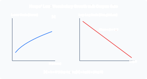
      Heaps' Law: vocabulary size vs corpus size on linear and log-log scales showing slope beta

      As a corpus grows, its vocabulary keeps growing, but with diminishing returns. No matter how much text you collect, you will always encounter new word types.

      V=k×Nβ\lvert V \rvert = k \times N^\beta

      • V\lvert V \rvert: vocabulary size (number of unique types)
      • NN: total number of tokens in the corpus
      • β\beta: exponent, typically 0.4-0.6
      • kk: language-dependent constant, typically 30-100

      Log-Log Estimation

      Taking logs:

      logV=log(k)+βlog(N)\log\lvert V \rvert = \log(k) + \beta \cdot \log(N)

      Plot log(vocabulary size)\log(\text{vocabulary size}) against log(total tokens)\log(\text{total tokens}). The result is a straight line:

      • Slope = β\beta
      • Y-intercept = log(k)\log(k)

      Why Growth Diminishes

      When only 100 tokens have been seen, each new token is likely to be a new type. After 10,000 tokens, most new tokens are repeats of known words. After 1 million tokens, genuinely new types are rare. Yet mathematically, V\lvert V \rvert never plateaus: it grows as NβN^\beta, which is unbounded (albeit slowly).

      With β=0.5\beta = 0.5: doubling NN increases V\lvert V \rvert by a factor of 20.51.412^{0.5} \approx 1.41. Quadrupling NN doubles V\lvert V \rvert.

      Heaps’ Law and Zipf’s Law: The Connection

      Zipf’s Law explains the shape of the frequency distribution (many rare words). Heaps’ Law explains the growth of vocabulary with corpus size (unbounded new types). Together they tell a single story: the tail of rare words is not only long but also inexhaustible. Collecting more data reduces but never eliminates the problem of unseen words.

      Consequence for Classification

      Smoothing is a mathematical necessity, not a pragmatic convenience. Heaps’ Law guarantees that:

      1. Any finite training corpus will have an incomplete vocabulary.
      2. New text will contain types never seen in training, regardless of training corpus size.
      3. Without smoothing, P(wc)=0P(w \mid c) = 0 for unseen words, collapsing all class probabilities to zero.

      This is the theoretical justification for Laplace (add-one) smoothing: it assigns non-zero probability to the infinite set of possible but unseen word types by reserving a portion of the probability mass.

      Summary

      AspectDetail
      Heaps’ LawV=k×Nβ\lvert V \rvert = k \times N^\beta
      β\beta range0.4-0.6
      kk range30-100
      EstimationLeast-squares on log-log plot
      ConsequenceVocabulary is effectively infinite; smoothing is mandatory

      Past paper questions: y2024p3q7 (feature engineering)

    • Naive Bayes Classification

      Core Idea

      Given a document dd and a set of classes CC, find the class with the highest posterior probability:

      c=argmaxcC P(cd)c^* = \underset{c \in C}{\text{argmax}} \ P(c \mid d)

      By Bayes’ Theorem:

      P(cd)=P(c)×P(dc)P(d)P(c \mid d) = \frac{P(c) \times P(d \mid c)}{P(d)}

      Since P(d)P(d) is constant across all classes for a given document, we drop it:

      c=argmaxcC P(c)×P(dc)c^* = \underset{c \in C}{\text{argmax}} \ P(c) \times P(d \mid c)

      The Naive Assumption

      The “naive” part: all features (words) are independent given the class. This lets us decompose the document probability into a product:

      P(dc)=i=1nP(wic)P(d \mid c) = \prod_{i=1}^{n} P(w_i \mid c)

      where w1,w2,,wnw_1, w_2, \dots, w_n are the words in the document. The full classification rule:

      c=argmaxcC P(c)×i=1nP(wic)c^* = \underset{c \in C}{\text{argmax}} \ P(c) \times \prod_{i=1}^{n} P(w_i \mid c)

      Parameter Estimation (Unsmoothed MLE)

      Prior:

      P(c)=NcNtotalP(c) = \frac{N_c}{N_{\text{total}}}

      where NcN_c is the number of training documents of class cc.

      Likelihood (Maximum Likelihood Estimate, no smoothing):

      P(wc)=count(w,c)wVcount(w,c)P(w \mid c) = \frac{\text{count}(w, c)}{\sum_{w' \in V} \text{count}(w', c)}

      where count(w,c)\text{count}(w, c) is the number of times word ww appears in documents of class cc, and VV is the vocabulary.

      The Zero-Probability Problem

      If any word ww in the test document never appeared with class cc in training, then count(w,c)=0\text{count}(w, c) = 0, so P(wc)=0P(w \mid c) = 0. The product P(wic)\prod P(w_i \mid c) becomes zero. If this happens for all classes, the classifier cannot decide.

      Even one unseen word kills the entire product. This is not a rare edge case: Zipf’s Law and Heaps’ Law guarantee that test documents will contain unseen words.

      Worked Example (Small 3-Word Problem)

      Training data (2 classes, SPAM and HAM):

      SPAM documents: “buy now”, “free buy” HAM documents: “meeting now”, “free lunch”

      Vocabulary V={buy,now,free,meeting,lunch}V = \{\text{buy}, \text{now}, \text{free}, \text{meeting}, \text{lunch}\}, V=5\lvert V \rvert = 5.

      Token counts per class:

      • SPAM: buy=2, now=1, free=1 (3 tokens total)
      • HAM: meeting=1, now=1, free=1, lunch=1 (4 tokens total)

      Priors: P(SPAM)=2/4=0.5P(\text{SPAM}) = 2/4 = 0.5, P(HAM)=2/4=0.5P(\text{HAM}) = 2/4 = 0.5.

      Likelihoods (unsmoothed):

      • P(buySPAM)=2/30.667P(\text{buy} \mid \text{SPAM}) = 2/3 \approx 0.667
      • P(buyHAM)=0/4=0P(\text{buy} \mid \text{HAM}) = 0/4 = 0 (never seen with HAM)

      Classify test document “buy lunch”:

      P(SPAM"buy lunch")0.5×(2/3)×P(lunchSPAM)P(\text{SPAM} \mid \text{"buy lunch"}) \propto 0.5 \times (2/3) \times P(\text{lunch} \mid \text{SPAM})

      P(lunchSPAM)=0/3=0P(\text{lunch} \mid \text{SPAM}) = 0/3 = 0 (never seen with SPAM).

      P(HAM"buy lunch")0.5×P(buyHAM)×(1/4)P(\text{HAM} \mid \text{"buy lunch"}) \propto 0.5 \times P(\text{buy} \mid \text{HAM}) \times (1/4)

      P(buyHAM)=0/4=0P(\text{buy} \mid \text{HAM}) = 0/4 = 0 (never seen with HAM).

      Both products collapse to zero. The classifier cannot choose. This is exactly what Laplace smoothing prevents.

      Interpretability

      Naive Bayes is interpretable: every parameter P(wc)P(w \mid c) is directly inspectable. If a feature value appears only with one class in training, you can identify the bias mathematically (e.g., P(Gender=FSuccess)=0P(\text{Gender=F} \mid \text{Success}) = 0 means the classifier can never predict Success for Female applicants). This property is invaluable for fairness auditing and is not available in black-box models.

      Summary

      ComponentFormulaNotes
      PriorP(c)=Nc/NtotalP(c) = N_c / N_{\text{total}}Fraction of training docs in class cc
      Likelihood (MLE)P(wc)=count(w,c)/count(w,c)P(w \mid c) = \text{count}(w,c) / \sum \text{count}(w',c)Zero for unseen words
      Classification rulec=argmaxc P(c)P(wic)c^* = \text{argmax}_c \ P(c) \prod P(w_i \mid c)Product collapses if any P(wic)=0P(w_i \mid c) = 0

      Past paper questions: y2021p3q9(a), y2023p3q8(a), y2024p3q9(a)

    • Laplace Add-One Smoothing

      The Problem

      Without smoothing, any word never seen with class cc in training gets P(wc)=0P(w \mid c) = 0. One unseen word makes the entire Naive Bayes product collapse to zero. Zipf’s Law and Heaps’ Law guarantee that unseen words are ubiquitous.

      Laplace (Add-One) Smoothing

      Add 1 to every word count and add V\lvert V \rvert to the denominator:

      P(wc)=count(w,c)+1wVcount(w,c)+VP(w \mid c) = \frac{\text{count}(w, c) + 1}{\sum_{w' \in V} \text{count}(w', c) + \lvert V \rvert}

      • V\lvert V \rvert: total number of unique word types across all training data (all classes combined)
      • Effect: shifts a small amount of probability mass from seen words to unseen ones
      • Every word type, even those never seen in training, now has P(wc)>0P(w \mid c) > 0

      General Smoothing Parameter ω\omega

      P(wc)=count(w,c)+ωwVcount(w,c)+ω×VP(w \mid c) = \frac{\text{count}(w, c) + \omega}{\sum_{w' \in V} \text{count}(w', c) + \omega \times \lvert V \rvert}

      Laplace smoothing is the special case ω=1\omega = 1. The parameter ω\omega can be tuned on the development set: try ω=0.1,0.5,1.0,2.0\omega = 0.1, 0.5, 1.0, 2.0 and pick the value that maximises dev-set accuracy or F1.

      Worked Example

      Revisiting the small 2-class problem from the Naive Bayes note.

      Training data:

      • SPAM documents: “buy now”, “free buy”
      • HAM documents: “meeting now”, “free lunch”

      Vocabulary V={buy,now,free,meeting,lunch}V = \{\text{buy}, \text{now}, \text{free}, \text{meeting}, \text{lunch}\}, V=5\lvert V \rvert = 5.

      Smoothed likelihoods:

      SPAM class (total tokens = 3):

      P(buySPAM)=2+13+5=38=0.375P(\text{buy} \mid \text{SPAM}) = \frac{2 + 1}{3 + 5} = \frac{3}{8} = 0.375

      P(nowSPAM)=1+13+5=28=0.25P(\text{now} \mid \text{SPAM}) = \frac{1 + 1}{3 + 5} = \frac{2}{8} = 0.25

      P(freeSPAM)=1+13+5=28=0.25P(\text{free} \mid \text{SPAM}) = \frac{1 + 1}{3 + 5} = \frac{2}{8} = 0.25

      P(meetingSPAM)=0+13+5=18=0.125P(\text{meeting} \mid \text{SPAM}) = \frac{0 + 1}{3 + 5} = \frac{1}{8} = 0.125

      P(lunchSPAM)=0+13+5=18=0.125P(\text{lunch} \mid \text{SPAM}) = \frac{0 + 1}{3 + 5} = \frac{1}{8} = 0.125

      HAM class (total tokens = 4):

      P(meetingHAM)=1+14+5=290.222P(\text{meeting} \mid \text{HAM}) = \frac{1 + 1}{4 + 5} = \frac{2}{9} \approx 0.222

      P(nowHAM)=1+14+5=290.222P(\text{now} \mid \text{HAM}) = \frac{1 + 1}{4 + 5} = \frac{2}{9} \approx 0.222

      P(freeHAM)=1+14+5=290.222P(\text{free} \mid \text{HAM}) = \frac{1 + 1}{4 + 5} = \frac{2}{9} \approx 0.222

      P(lunchHAM)=1+14+5=290.222P(\text{lunch} \mid \text{HAM}) = \frac{1 + 1}{4 + 5} = \frac{2}{9} \approx 0.222

      P(buyHAM)=0+14+5=190.111P(\text{buy} \mid \text{HAM}) = \frac{0 + 1}{4 + 5} = \frac{1}{9} \approx 0.111

      Classify “buy lunch”:

      Priors: P(SPAM)=0.5P(\text{SPAM}) = 0.5, P(HAM)=0.5P(\text{HAM}) = 0.5.

      P(SPAMd)0.5×0.375×0.125=0.5×0.046875=0.02344P(\text{SPAM} \mid d) \propto 0.5 \times 0.375 \times 0.125 = 0.5 \times 0.046875 = 0.02344

      P(HAMd)0.5×0.111×0.222=0.5×0.02464=0.01232P(\text{HAM} \mid d) \propto 0.5 \times 0.111 \times 0.222 = 0.5 \times 0.02464 = 0.01232

      The classifier predicts SPAM. Without smoothing, both products were zero; the classifier could not choose. With Laplace smoothing, every word has non-zero probability, and the classifier works correctly.

      Exam Rule

      Apply smoothing whenever the question does not explicitly say “without smoothing”. Always state V\lvert V \rvert explicitly as the denominator correction.

      Summary

      SmoothingFormulaω\omega
      Laplace (add-one)(count+1)/(total+V)(\text{count}+1) / (\text{total}+\lvert V \rvert)1
      Add-ω\omega (general)(count+ω)/(total+ωV)(\text{count}+\omega) / (\text{total}+\omega\lvert V \rvert)Tuned on dev set

      Past paper questions: y2021p3q9(a), y2023p3q8(a), y2024p3q9(a)

    • Log-Probability and Underflow Mitigation

      The Underflow Problem

      The Naive Bayes classification rule multiplies many small probabilities:

      P(c)×i=1nP(wic)P(c) \times \prod_{i=1}^{n} P(w_i \mid c)

      With Laplace smoothing, a typical P(wc)P(w \mid c) might be ~0.001. For a document with 100 words, the product is roughly (103)100=10300(10^{-3})^{100} = 10^{-300}. Standard 64-bit floating-point numbers can represent values down to approximately 1030810^{-308} before hitting zero. A 100-word document is close to this boundary; longer documents or smaller probabilities push the product to exactly zero on the computer.

      Floating-point underflow turns a mathematically valid (but tiny) number into zero. When this happens, the classifier loses all discriminative information: every class product becomes zero, and the argmax is meaningless.

      Solution: Work in Log Space

      Since log\log is strictly monotonically increasing, the argmax is identical:

      c=argmaxcC log(P(c)×i=1nP(wic))c^* = \underset{c \in C}{\text{argmax}} \ \log\left(P(c) \times \prod_{i=1}^{n} P(w_i \mid c)\right)

      c=argmaxcC [logP(c)+i=1nlogP(wic)]c^* = \underset{c \in C}{\text{argmax}} \ \left[ \log P(c) + \sum_{i=1}^{n} \log P(w_i \mid c) \right]

      The product becomes a sum of log-probabilities. Each logP(wc)\log P(w \mid c) is a moderate negative number (e.g., log(0.001)=6.91\log(0.001) = -6.91). For 100 words, the sum is roughly 691-691, which is easily representable.

      Why This Works

      Logarithms map multiplication to addition:

      log(a×b)=log(a)+log(b)\log(a \times b) = \log(a) + \log(b)

      For three probabilities:

      log(P(c)×P(w1c)×P(w2c))=logP(c)+logP(w1c)+logP(w2c)\log(P(c) \times P(w_1 \mid c) \times P(w_2 \mid c)) = \log P(c) + \log P(w_1 \mid c) + \log P(w_2 \mid c)

      Each term is a negative number. The sum grows (becomes more negative) linearly with document length, rather than exponentially shrinking toward zero.

      Worked Example

      Classify a 10-word document with two classes. Smoothed probabilities:

      WordP(wClass A)P(w \mid \text{Class A})P(wClass B)P(w \mid \text{Class B})
      w1w_10.0010.002
      w2w_20.0030.001
      w3w_30.00050.004
      w4w_40.0020.001
      w5w_50.0010.003
      w6w_60.0040.0005
      w7w_70.0010.002
      w8w_80.0020.001
      w9w_90.0030.001
      w10w_{10}0.00050.002

      Priors: P(A)=0.6P(\text{A}) = 0.6, P(B)=0.4P(\text{B}) = 0.4.

      In probability space (dangerous):

      P(Ad)0.6×(0.001×0.003×0.0005×)P(\text{A} \mid d) \propto 0.6 \times (0.001 \times 0.003 \times 0.0005 \times \dots)

      The product is approximately 103410^{-34}, still representable for 10 words, but for 100 words it would underflow.

      In log space (safe):

      logP(A)=log(0.6)=0.511\log P(\text{A}) = \log(0.6) = -0.511

      logP(wiA)=log(0.001)+log(0.003)+log(0.0005)+=6.908+(5.809)+(7.601)+\sum \log P(w_i \mid \text{A}) = \log(0.001) + \log(0.003) + \log(0.0005) + \dots = -6.908 + (-5.809) + (-7.601) + \dots

      Sum for A: 0.511+(65.2)=65.7-0.511 + (-65.2) = -65.7. Sum for B: log(0.4)+(58.4)=0.916+(58.4)=59.3\log(0.4) + (-58.4) = -0.916 + (-58.4) = -59.3.

      Since 59.3>65.7-59.3 > -65.7, the classifier predicts Class B. The log-space computation is numerically stable for documents of any length.

      Implementation Note

      Always convert to log space immediately after computing smoothed probabilities. Pre-compute logP(wc)\log P(w \mid c) for every word-class pair during training. At classification time, sum the pre-computed log values for the words in the document and add logP(c)\log P(c). The class with the largest (least negative) sum wins.

      Summary

      ApproachOperationRisk
      Probability spaceMultiply P(wc)P(w \mid c)Underflow for ~100+ words
      Log spaceSum logP(wc)\log P(w \mid c)Safe for any document length

      Past paper questions: y2021p3q9(a)

    • Feature Engineering and Generalisation

      Why Feature Engineering Matters

      Raw text produces a sparse, high-dimensional feature space. Naive Bayes’ independence assumption becomes less tenable, and zero-probability events proliferate. Feature engineering reduces sparsity and improves generalisation to unseen data.

      Lowercasing

      Convert all text to lowercase: “Running” and “running” become the same type.

      Why it helps: Reduces vocabulary size without losing discriminative information. Capitalisation rarely carries class-relevant signal in standard text classification. A halved vocabulary means fewer unseen-word events and more reliable probability estimates per type.

      Stemming and Lemmatisation

      Map morphological variants to a common root:

      • “argued”, “arguing”, “argues”, “argument” → “argu” (stemming)
      • “better”, “good” → “good” (lemmatisation, handles irregular forms)

      Why it helps: Groups related forms together, increasing the count for each root and reducing vocabulary size. The probability estimate for “argu” is based on the combined evidence from all its surface forms, making it more reliable.

      Stop-Word Removal

      Remove high-frequency function words: “the”, “and”, “is”, “of”, “to”, “a”.

      Why it helps: These words appear in every document regardless of class. They carry no discriminative power and add noise. Removing them reduces document length and vocabulary size without affecting the classifier’s ability to separate classes.

      Hapax Legomena Removal

      Remove words that occur exactly once in the training data (hapax legomena, singular: hapax legomenon).

      Why it helps: A word seen only once provides an unreliable probability estimate. It may be a typo, a rare proper noun, or statistical noise. Removing hapaxes reduces vocabulary size and prevents the classifier from overfitting to idiosyncratic training tokens that will never appear again. The trade-off: some rare but genuinely informative words are lost, but the noise reduction usually outweighs this.

      Binning Continuous Features

      For numerical features (age, income, scores), group values into discrete brackets:

      • Age 18, 19, 20 → [17-20]
      • Score 72, 88, 91 → [70-80], [80-90], [90-100]

      Why it helps: Naive Bayes requires discrete features. A continuous feature like age has potentially infinite values, each with zero or negligible counts. Binning reduces the feature to a small set of categories, each with meaningful probability estimates. The bracket width can be tuned on the development set.

      Lexicon Integration

      Replace specific words with generic sentiment tokens:

      • “awful”, “terrible”, “dreadful” → <NEGATIVE_WORD>
      • “excellent”, “wonderful”, “brilliant” → <POSITIVE_WORD>

      Why it helps: Unseen synonyms of known sentiment words are mapped to the same token, so the classifier recognises their polarity even without having seen the specific word in training. This handles language change and domain shift: a new slang term for “bad” is still replaced by <NEGATIVE_WORD> if it appears in the lexicon.

      Combined Approach

      These techniques are not mutually exclusive. A typical pipeline: lowercase → remove stop words → stem → remove hapaxes → replace lexicon words with polarity tokens. The development set guides which combination produces the best held-out performance.

      Summary

      TechniqueWhat it doesWhy it helps
      Lowercasing”Running” → “running”Halves vocabulary, same discriminative power
      Stemming/lemmatisation”argued”/“arguing” → “argu”Groups variants, more reliable counts
      Stop-word removalDrop “the”, “and”, “is”Removes non-discriminative noise
      Hapax removalDrop words seen onceRemoves unreliable probability estimates
      BinningAge 18 → [17-20]Reduces sparsity for numerical features
      Lexicon integration”awful” → <NEGATIVE_WORD>Handles unseen synonyms, language change

      Past paper questions: y2021p3q9(c)(ii), y2021p3q9(e)(iii), y2024p3q7(d)

  • Naive Bayes: Bias, Interpretability, and Lexicons

    Detecting and proving bias in Naive Bayes classifiers, non-interpretable vs interpretable models, and combining Naive Bayes with lexicon-based approaches

    • Detecting and Proving Bias in Naive Bayes

      Why Naive Bayes Is Interpretable

      Naive Bayes is interpretable: you can inspect every parameter — every P(wc)P(w \mid c), every P(c)P(c) — directly from the probability table. You can trace any classification decision back to which specific features contributed which specific probabilities.

      The useful property: identify bias immediately by scanning the parameter table for zeros. If P(featureclass)=0P(\text{feature} \mid \text{class}) = 0, that class can never be predicted when that feature is present. You can prove this mathematically with two test instances.

      The problematic property: zero probabilities propagate. Multiplying small probabilities together means one zero anywhere in the product makes the entire posterior zero — the classifier becomes completely insensitive to all other evidence. A single unseen word or feature value kills the classifier for that instance.

      This interpretability is impossible with black-box models (neural networks, random forests, SVMs). You cannot inspect individual parameters, trace decisions to specific training examples, or construct guaranteed counter-examples.

      The 4-Step Method for Proving Bias

      To mathematically demonstrate that a classifier is biased against a protected group:

      1. Identify a protected attribute (Gender, Ethnicity, Nationality, Age).
      2. Find a value of that attribute that only appears in one class in the training data (i.e., P(valueother_class)=0P(\text{value} \mid \text{other\_class}) = 0).
      3. Construct two identical test instances differing ONLY in the protected attribute. All other features should appear in both classes (neutral features).
      4. Show that the classifier gives different predictions for the two instances, or show P(classprotected_value)=0P(\text{class} \mid \text{protected\_value}) = 0, meaning that class can NEVER be predicted for any instance with that protected value — regardless of all other features.

      Full Worked Example: Football Academy (2024 Q9)

      Training data: 6 recruits with features Goals (Many/Few/None), Position (Attack/Defender/Goalkeeper), Gender (M/F), and label Success (Y/N).

      Step 1 — Priors

      P(Y)=36=0.5P(N)=36=0.5P(Y) = \frac{3}{6} = 0.5 \qquad P(N) = \frac{3}{6} = 0.5

      Step 2 — Likelihoods (MLE, no smoothing)

      Goals:

      P(ManyY)=13P(FewY)=13P(NoneY)=13P(\text{Many} \mid Y) = \frac{1}{3} \quad P(\text{Few} \mid Y) = \frac{1}{3} \quad P(\text{None} \mid Y) = \frac{1}{3}

      P(ManyN)=0P(FewN)=23P(NoneN)=13P(\text{Many} \mid N) = 0 \quad P(\text{Few} \mid N) = \frac{2}{3} \quad P(\text{None} \mid N) = \frac{1}{3}

      Position:

      P(AttackY)=23P(DefenderY)=13P(GoalkeeperY)=0P(\text{Attack} \mid Y) = \frac{2}{3} \quad P(\text{Defender} \mid Y) = \frac{1}{3} \quad P(\text{Goalkeeper} \mid Y) = 0

      P(AttackN)=0P(DefenderN)=23P(GoalkeeperN)=13P(\text{Attack} \mid N) = 0 \quad P(\text{Defender} \mid N) = \frac{2}{3} \quad P(\text{Goalkeeper} \mid N) = \frac{1}{3}

      Gender:

      P(MY)=1P(FY)=0P(\text{M} \mid Y) = 1 \quad P(\text{F} \mid Y) = 0 P(MN)=23P(FN)=13P(\text{M} \mid N) = \frac{2}{3} \quad P(\text{F} \mid N) = \frac{1}{3}

      Bias Group 1: Goalkeepers (Protected: Position)

      Protected value: Position = Goalkeeper. Only appears with class N in training.

      Test instance: Goals=None, Position=Goalkeeper, Gender=M.

      P(Yinstance)P(Y)P(NoneY)P(GoalkeeperY)P(MY)P(Y \mid \text{instance}) \propto P(Y) \cdot P(\text{None} \mid Y) \cdot P(\text{Goalkeeper} \mid Y) \cdot P(\text{M} \mid Y) =0.51301=0= 0.5 \cdot \frac{1}{3} \cdot 0 \cdot 1 = 0

      A Goalkeeper can NEVER be predicted as Successful — regardless of their Goals scored or Gender. The zero from P(GoalkeeperY)P(\text{Goalkeeper} \mid Y) propagates through the product and wipes out all other information.

      Bias Group 2: Female Players (Protected: Gender)

      Protected value: Gender = F. Only appears with class N in training.

      Test instance: Goals=Many, Position=Attack, Gender=F.

      P(Yinstance)0.513230=0P(Y \mid \text{instance}) \propto 0.5 \cdot \frac{1}{3} \cdot \frac{2}{3} \cdot 0 = 0

      A Female player can NEVER be predicted as Successful — regardless of their Goals or Position. Every P(Y)P(Y \mid \dots) is zero the moment Gender=F appears.

      Why This Happened

      The training data encoded historical discrimination: no Female players and no Goalkeepers appeared in the Successful group. Naive Bayes faithfully reproduced the patterns in the data. This mirrors the London Medical School Admissions case: a program built to replicate human admissions decisions reproduced the gender and ethnic discrimination present in the historical training data. “Fitting the data” does not produce fair decisions if the data itself reflects historical injustice.

      Summary

      ConceptKey Point
      InterpretabilityEvery P(wc)P(w \mid c) is directly inspectable — impossible with black-box models
      Zero propagationOne zero in the NB product kills all classification power
      4-step proofProtected attribute → find exclusive value → construct test pair → show inequality
      Goalkeeper biasP(GoalkeeperY)=0P(\text{Goalkeeper} \mid Y) = 0, can never predict Y
      Gender biasP(FY)=0P(\text{F} \mid Y) = 0, can never predict Y
      Root causeHistorical discrimination encoded in training data; NB faithfully reproduces it

      Past paper questions: y2024p3q9

    • Naive Bayes versus Lexicon-Based Approaches

      Two Approaches to Text Classification

      Naive Bayes is a supervised statistical classifier: it learns P(wc)P(w \mid c) from labelled training data by counting word-class co-occurrences. The decision rule is:

      c=argmaxc  P(c)i=1nP(wic)c^* = \arg\max_{c} \; P(c) \prod_{i=1}^{n} P(w_i \mid c)

      Lexicon-based classification uses a hand-built dictionary where each word has a pre-assigned polarity or category (e.g., “terrible” → negative, “great” → positive). The decision is typically a sum or majority vote over lexicon matches. No training data is needed.

      When Naive Bayes Wins

      Naive Bayes is the better choice when:

      • Sufficient labelled training data exists. The classifier needs enough examples per class to estimate reliable word probabilities. With thousands of labelled messages, NB can detect subtle statistical patterns.
      • Statistical patterns capture subtle discrimination. Combinations of seemingly neutral words (e.g., “you should know your place”) can together signal bullying even though no individual word is in a bullying lexicon. NB captures these co-occurrence patterns.
      • Domain language differs from standard lexicons. A general sentiment lexicon performs poorly on specialised domains like gaming slang, medical reports, or legal documents. NB learns the domain-specific vocabulary directly from the labelled data.

      When Lexicon-Based Wins

      A lexicon is better when:

      • Very little labelled data is available. Building a domain lexicon requires modest expert effort but no labelled examples.
      • The domain is well-covered by existing lexicons. Sentiment analysis with standard dictionaries (LIWC, VADER, SentiWordNet) needs no training data.
      • You need explicit, inspectable rules. A human can read the lexicon and understand exactly which words trigger which decisions. This is essential in regulated settings where decisions must be explainable and auditable.

      The Best-of-Both Strategy

      Use lexicon tokens as Naive Bayes features: replace specific words with generic category tokens before training.

      Original textAfter lexicon preprocessing
      ”you are awful and ugly""you are <NEGATIVE> and <NEGATIVE>"
      "that is brilliant work""that is <POSITIVE> work”

      This hybrid approach provides four advantages:

      • Handles unseen synonyms: if “grotesque” is in the lexicon but never appeared in training, it maps to <NEGATIVE> and NB can use it immediately.
      • Handles language change: new bullying slang (e.g., “ratio’d”, “mid”) can be added to the lexicon without retraining the full NB model.
      • Reduces vocabulary size dramatically: all positive words collapse into one feature, all negative words into another. The vocabulary V|V| shrinks, reducing the zero-probability problem and improving smoothing.
      • Combines strengths: NB captures word co-occurrence and overall message tone; the lexicon captures expert knowledge about specific words and handles the long tail.

      Cyberbullying Detection Example (2021 Q9)

      In cyberbullying detection, language change is the critical threat. Younger users constantly invent new words and repurpose existing ones. A fixed NB classifier degrades rapidly.

      Building a Cyberbullying Lexicon

      Method 1 (new words): track unknown words during classification. If a word suddenly spikes in frequency, sample messages containing it, have them manually labelled, and add the word to the lexicon if bullying-related. The labelled messages become new training data.

      Method 2 (new senses): find “maximally surprising” messages where the classifier was confident but wrong. Check whether known words in these messages have acquired a new threatening sense. Add these to the lexicon and use the surprising messages for retraining.

      Robustness to Language Change

      Run the lexicon-based detector on new messages to cheaply identify likely bullying instances. Use these as new training material for periodic NB retraining. The lexicon acts as a lightweight, continuously-updated scout. Active learning approaches can also help: find the messages where the classifier is most uncertain, have humans label those, and retrain NB.

      Evaluation with Lexicons

      When a company policy demands “delete as many bullying messages as possible while keeping non-filtered messages high,” this translates to: optimise recall (find all bullying) while maintaining reasonable precision (don’t falsely flag OK messages). Precision and recall — not accuracy — are the right metrics because bullying messages are rare, and accuracy would be dominated by correctly identifying the abundant OK messages. A development corpus helps find the probability threshold that balances precision and recall for the new policy.

      Comparison Summary

      CriterionNaive BayesLexicon
      Requires labelled dataYes, substantialNo
      Handles unseen wordsVia smoothingIf word is in lexicon
      Handles language changePoorly (needs retraining)Well (update lexicon)
      Captures subtle patternsYes (co-occurrence)No (word-level only)
      InterpretabilityInspectable parametersExplicit rules
      Domain adaptationLearns from dataRequires domain lexicon
      Best-of-bothLexicon tokens as NB featuresBridges both worlds

      Past paper questions: y2021p3q9, y2025p3q7

  • Hidden Markov Models

    HMM definition, the three assumptions, parameter estimation with smoothing, the Viterbi decoding algorithm, common shortcomings, and time-aware compound states

    • Hidden Markov Models: Definition

      Motivation

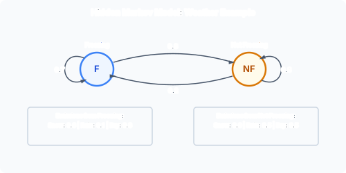
      Two-state weather HMM with transitions between Freezing and Not Freezing states, showing emission probabilities for each state

      Naive Bayes treats every observation independently: word order does not matter. But many real-world problems involve sequences where items depend on their neighbours: speech, weather patterns, financial time series, biological sequences (DNA, proteins). Hidden Markov Models explicitly model these temporal dependencies through a two-level structure: hidden states that evolve over time and visible observations emitted by those states.

      Formal Definition: μ=(S,V,A,B,π)\mu = (S, V, A, B, \pi)

      An HMM models a system where we observe outputs (emissions) but cannot directly observe the underlying process (hidden states). The model is fully specified by five components:

      SymbolNameDescription
      SSHidden StatesThe unobservable states: $S = {s_1, s_2, \ldots, s_{
      VVObservationsThe observable emissions: $V = {v_1, v_2, \ldots, v_{
      AATransition Matrixaij=P(qt=sjqt1=si)a_{ij} = P(q_t = s_j \mid q_{t-1} = s_i) — row ii, column jj
      BBEmission Matrixbi(vk)=P(ot=vkqt=si)b_i(v_k) = P(o_t = v_k \mid q_t = s_i) — row ii, column kk
      π\piInitial Distributionπj=P(q1=sj)\pi_j = P(q_1 = s_j) — probability of starting in state jj

      Each row of AA sums to 1. Each row of BB sums to 1. jπj=1\sum_j \pi_j = 1.

      Concrete Example: Weather HMM

      This is the 2024 Q8 HMM. Hidden states: S={Freezing(F),NotFreezing(NF)}S = \{\text{Freezing}(F), \text{NotFreezing}(NF)\} (air temperature, unobservable without a thermometer). Observations: V={Snow(S),Rain(R),Dry(D)}V = \{\text{Snow}(S), \text{Rain}(R), \text{Dry}(D)\} (visible weather).

      Transition matrix AA — models how temperature changes month to month:

      qt1q_{t-1} / qtq_tFFNFNF
      FFP(FF)P(F \mid F)P(NFF)P(NF \mid F)
      NFNFP(FNF)P(F \mid NF)P(NFNF)P(NF \mid NF)

      Emission matrix BB — models the weather given the temperature:

      qtq_t / oto_tSSRRDD
      FFP(SF)P(S \mid F)P(RF)P(R \mid F)P(DF)P(D \mid F)
      NFNFP(SNF)P(S \mid NF)P(RNF)P(R \mid NF)P(DNF)P(D \mid NF)

      Note: Snow requires freezing temperatures (P(SNF)0P(S \mid NF) \approx 0). Rain implies above-freezing (P(RF)0P(R \mid F) \approx 0). Dry is possible in either state.

      Initial distribution π\pi: π=[P(q1=F),  P(q1=NF)]\pi = [P(q_1 = F),\; P(q_1 = NF)].

      What Makes HMMs Different from Naive Bayes

      Naive Bayes: P(cd)P(c)iP(wic)P(c \mid d) \propto P(c) \prod_i P(w_i \mid c) — each word contributes independently. Word order does not matter. “The dog bit the man” and “The man bit the dog” are identical to NB.

      HMMs model the dependence between consecutive items through the transition matrix AA. The hidden state at time tt depends on the hidden state at t1t-1. The observation at time tt depends on the state at tt. This sequential structure makes HMMs suitable for any data where context matters: part-of-speech tagging, speech recognition, activity recognition, financial regime detection.

      Dual-Tape Training Data

      Training requires fully labelled sequences: both the hidden state and the observation at every timestep must be known. This is called dual-tape data. Example:

      Timestep1234567
      State (qtq_t)LMHHHMM
      Observation (oto_t)+++++++++++++

      From this we count transitions and emissions to estimate AA and BB.

      Summary

      ComponentFormulaMeaning
      SSSet of hidden states (size $
      VVSet of observable symbols (size $
      aija_{ij}P(qt=sjqt1=si)P(q_t = s_j \mid q_{t-1} = s_i)Transition probability
      bi(vk)b_i(v_k)P(ot=vkqt=si)P(o_t = v_k \mid q_t = s_i)Emission probability
      πj\pi_jP(q1=sj)P(q_1 = s_j)Initial state probability
      Rows sum to 1jaij=1\sum_j a_{ij} = 1, kbi(vk)=1\sum_k b_i(v_k) = 1Valid probability distributions

      Past paper questions: y2024p3q8, y2025p3q9

    • Hidden Markov Models: The Three Assumptions

      Exam Context

      This sub-question appears every year. You must state all three assumptions explicitly, give their formal mathematical form, and evaluate each in the context of the specific application given in the question. Generic statements without evaluation lose marks. Each assumption typically earns 1 mark for stating it plus 1 mark for contextual evaluation.

      The Three Assumptions

      1. First-Order Markov Assumption

      P(qtq1,q2,,qt1)=P(qtqt1)P(q_t \mid q_1, q_2, \ldots, q_{t-1}) = P(q_t \mid q_{t-1})

      Only the immediately preceding state matters. The entire history before t1t-1 is irrelevant once qt1q_{t-1} is known. This means the transition matrix AA needs only S×S|S| \times |S| entries rather than growing exponentially with the sequence length.

      Fails when: trends depend on longer history. Multi-day weather patterns (a cold front lasting a week), economic cycles (a recession spanning quarters), or infection waves where the path from low to high typically passes through medium over multiple timesteps. A first-order model cannot distinguish “the first cold day of an autumn cold snap” from “the tenth consecutive freezing day of a deep winter freeze” — both cases have the same P(FF)P(F \mid F) transition, but the probability of continuing freezing is very different.

      2. Output Independence Assumption

      P(otq1,,qt,o1,,ot1)=P(otqt)P(o_t \mid q_1, \ldots, q_t, o_1, \ldots, o_{t-1}) = P(o_t \mid q_t)

      The observation at time tt depends solely on the current hidden state qtq_t. All previous states, future states, and all other observations are irrelevant once qtq_t is known. This means bi(vk)b_i(v_k) captures everything about oto_t.

      Fails when: consecutive observations are correlated beyond what the hidden state explains. If it rained today, rain is more likely tomorrow — regardless of whether the hidden temperature state has changed. In speech recognition, neighbouring phonemes influence each other acoustically (coarticulation): the sound of /t/ differs depending on whether the next phoneme is /i/ or /u/. In part-of-speech tagging, an adjective is more likely to be followed by a noun regardless of any hidden syntactic state.

      3. Stationarity Assumption

      P(qt=sjqt1=si) and P(ot=vkqt=si) are constant for all tP(q_t = s_j \mid q_{t-1} = s_i) \text{ and } P(o_t = v_k \mid q_t = s_i) \text{ are constant for all } t

      Transition probabilities AA and emission probabilities BB do not change over time. The same matrices apply whether t=1t = 1, t=100t = 100, or t=1000t = 1000.

      Fails when: behaviour is seasonal (summer vs. winter transitions differ), structural (policy changes alter relationships between states and observations), or evolutionary (language changes over decades, market regimes shift gradually). For the 2024 weather HMM: P(NFF)P(NF \to F) in October (heading into winter) is far higher than P(NFF)P(NF \to F) in March (heading into spring). The stationary model averages these into a single number that overestimates freezing probability in summer and underestimates it in winter.

      Evaluating in Context: COVID HMM (2022 Q9)

      For an infection-level HMM with hidden states {L,M,H}\{L, M, H\}:

      1. First-order Markov: infection levels follow multi-week trends (a wave building over a month). The probability of staying at H may depend on how many consecutive H weeks have already elapsed — the model cannot capture this duration dependence. First-order is probably too short a memory.

      2. Output independence: consecutive test positivity rates are likely correlated. A testing centre with high positivity one week tends to have high positivity the next, independent of whether the true infection level changed, due to consistent testing demographics and reporting lags (the same people retested, the same labs processing). This violates output independence.

      3. Stationarity: COVID behaviour changed dramatically between variants (Alpha, Delta, Omicron). Each variant had different transmission dynamics, different incubation periods, and different relationships between infection prevalence and test positivity. A model estimated from early-2020 data would produce wrong predictions on late-2021 data because the underlying process had changed.

      Summary

      AssumptionFormal StatementTypical Failure Mode
      First-order MarkovP(qtqt1)P(q_t \mid q_{t-1}) only; history before t1t-1 irrelevantTrends persist over multiple timesteps (multi-week fronts)
      Output independenceP(otqt)P(o_t \mid q_t) only; all other observations irrelevantConsecutive observations are correlated (rain clustering)
      StationarityA,BA, B invariant for all ttSeasons, policy shifts, variant emergence, regime changes

      Past paper questions: y2022p3q9, y2024p3q8, y2025p3q9

    • Hidden Markov Models: Parameter Estimation and Smoothing

      Maximum Likelihood Estimation (MLE, no smoothing)

      From fully labelled training data (dual-tape), count and divide:

      Transitions:

      aij=count(sisj)count(si)a_{ij} = \frac{\text{count}(s_i \to s_j)}{\text{count}(s_i)}

      Emissions:

      bi(vk)=count(si emits vk)count(si)b_i(v_k) = \frac{\text{count}(s_i \text{ emits } v_k)}{\text{count}(s_i)}

      Problem: any count of zero gives probability zero. In Viterbi decoding, a zero anywhere kills that path entirely. With small training sets, many transitions and emissions will be unseen.

      Laplace (Add-One) Smoothing

      Transitions:

      aij=count(sisj)+1count(si)+Sa_{ij} = \frac{\text{count}(s_i \to s_j) + 1}{\text{count}(s_i) + |S|}

      Emissions:

      bi(vk)=count(si emits vk)+1count(si)+Vb_i(v_k) = \frac{\text{count}(s_i \text{ emits } v_k) + 1}{\text{count}(s_i) + |V|}

      CRITICAL: Denominators Are Different

      This is the most common exam error. Transitions add S|S| (number of hidden states) to the denominator. Emissions add V|V| (number of observation symbols) to the denominator. They are different quantities and students who mix them up lose marks.

      Why they differ: a transition goes to one of S|S| possible next states, so we smooth across S|S| outcomes. An emission goes to one of V|V| possible observation symbols, so we smooth across V|V| outcomes.

      Full Worked Example: COVID HMM (2022 Q9)

      Training Data (timesteps 1–7)

      States: L, M, H, H, H, M, M Observations: +, ++, ++, +++, ++, ++, +

      Counting Transitions

      From / ToLMH
      L010
      M021
      H012

      count(L)=1\text{count}(L) = 1, count(M)=3\text{count}(M) = 3, count(H)=3\text{count}(H) = 3

      Without smoothing:

      aLM=11=1.0aMH=13aMM=23a_{L \to M} = \frac{1}{1} = 1.0 \quad a_{M \to H} = \frac{1}{3} \quad a_{M \to M} = \frac{2}{3} aHH=23aHM=13aLL=01=0a_{H \to H} = \frac{2}{3} \quad a_{H \to M} = \frac{1}{3} \quad a_{L \to L} = \frac{0}{1} = 0

      aLL=0a_{L \to L} = 0 is problematic: if we ever reach state L, we cannot stay there.

      With smoothing (S=3|S| = 3):

      aLM=1+11+3=24aMH=1+13+3=26a_{L \to M} = \frac{1+1}{1+3} = \frac{2}{4} \quad a_{M \to H} = \frac{1+1}{3+3} = \frac{2}{6} aMM=2+13+3=36aHH=2+13+3=36a_{M \to M} = \frac{2+1}{3+3} = \frac{3}{6} \quad a_{H \to H} = \frac{2+1}{3+3} = \frac{3}{6} aHM=1+13+3=26aLL=0+11+3=14a_{H \to M} = \frac{1+1}{3+3} = \frac{2}{6} \quad a_{L \to L} = \frac{0+1}{1+3} = \frac{1}{4}

      Counting Emissions

      State / Obs++++++
      L100
      M030
      H012

      count(L)=1\text{count}(L) = 1, count(M)=3\text{count}(M) = 3, count(H)=3\text{count}(H) = 3

      Without smoothing:

      bL(+)=11=1.0bM(++)=33=1.0bH(++)=13bH(+++)=23b_L(+) = \frac{1}{1} = 1.0 \quad b_M(\text{++}) = \frac{3}{3} = 1.0 \quad b_H(\text{++}) = \frac{1}{3} \quad b_H(\text{+++}) = \frac{2}{3}

      Zeros everywhere: bL(++)=0b_L(\text{++}) = 0, bL(+++)=0b_L(\text{+++}) = 0, bM(+)=0b_M(+) = 0, bM(+++)=0b_M(\text{+++}) = 0, bH(+)=0b_H(+) = 0.

      With smoothing (V=3|V| = 3):

      bL(+)=1+11+3=24bM(++)=3+13+3=46bH(+++)=2+13+3=36b_L(+) = \frac{1+1}{1+3} = \frac{2}{4} \quad b_M(\text{++}) = \frac{3+1}{3+3} = \frac{4}{6} \quad b_H(\text{+++}) = \frac{2+1}{3+3} = \frac{3}{6}

      General Smoothing Parameter ω\omega

      aij=count(sisj)+ωcount(si)+ωSa_{ij} = \frac{\text{count}(s_i \to s_j) + \omega}{\text{count}(s_i) + \omega \cdot |S|}

      bi(vk)=count(si emits vk)+ωcount(si)+ωVb_i(v_k) = \frac{\text{count}(s_i \text{ emits } v_k) + \omega}{\text{count}(s_i) + \omega \cdot |V|}

      Laplace smoothing is the special case ω=1\omega = 1. ω\omega can be tuned on a development set (cross-validation).

      Summary

      QuantityMLE (no smoothing)Laplace (add-one)
      aija_{ij}count(sisj)count(si)\frac{\text{count}(s_i \to s_j)}{\text{count}(s_i)}count(sisj)+1count(si)+S\frac{\text{count}(s_i \to s_j) + 1}{\text{count}(s_i) + \|S\|}
      bi(vk)b_i(v_k)count(si emits vk)count(si)\frac{\text{count}(s_i \text{ emits } v_k)}{\text{count}(s_i)}count(si emits vk)+1count(si)+V\frac{\text{count}(s_i \text{ emits } v_k) + 1}{\text{count}(s_i) + \|V\|}
      Smoothing amountNoneShift mass from seen to unseen
      Most common errorAdding V\|V\| to transition denominator

      Past paper questions: y2022p3q9, y2024p3q8, y2025p3q9

    • The Viterbi Decoding Algorithm

      Purpose

      Viterbi finds the single most likely hidden-state sequence q1,q2,,qTq_1^*, q_2^*, \ldots, q_T^* given an observation sequence o1,o2,,oTo_1, o_2, \ldots, o_T. It is a dynamic programming algorithm: at each timestep, for each state, it stores the best path probability reaching that state and a backpointer.

      Components

      δj(t)\delta_j(t): the probability of the most likely path reaching state jj at time tt, accounting for observations o1o_1 through oto_t.

      ψj(t)\psi_j(t): the backpointer — which state at t1t-1 produced the best path to state jj at time tt.

      Algorithm

      Initialisation (t=1t = 1)

      For each state jj:

      δj(1)=πjbj(o1)ψj(1)=0\delta_j(1) = \pi_j \cdot b_j(o_1) \qquad \psi_j(1) = 0

      Recursion (t=2,3,,Tt = 2, 3, \dots, T)

      For each state jj:

      δj(t)=maxi[δi(t1)aijbj(ot)]\delta_j(t) = \max_i \big[ \delta_i(t-1) \cdot a_{ij} \cdot b_j(o_t) \big] ψj(t)=argmaxi[δi(t1)aij]\psi_j(t) = \arg\max_i \big[ \delta_i(t-1) \cdot a_{ij} \big]

      Note: bj(ot)b_j(o_t) is the same for all ii, so it can be pulled outside the max. The argmax\arg\max is over δi(t1)aij\delta_i(t-1) \cdot a_{ij} only.

      Termination (t=Tt = T)

      Best path probability: P=maxiδi(T)P^* = \max_i \delta_i(T)

      Final state: qT=argmaxiδi(T)q_T^* = \arg\max_i \delta_i(T)

      Backtracking (t=T1t = T-1 down to 11)

      qt=ψqt+1(t+1)q_t^* = \psi_{q_{t+1}^*}(t+1)

      Read the backpointer chain backwards to reconstruct the optimal state sequence.

      Trellis Layout

      Draw a grid: rows = states, columns = timesteps. Fill each cell with δj(t)\delta_j(t) and ψj(t)\psi_j(t). Circle the maximum in each column. Draw arrows from each cell to its backpointer source. After termination, trace arrows backwards from the final state.

      Log-Space Implementation

      In practice, use log-probabilities to prevent underflow:

      δj(t)=maxi[δi(t1)+logaij+logbj(ot)]\delta_j(t) = \max_i \big[ \delta_i(t-1) + \log a_{ij} + \log b_j(o_t) \big]

      Products become sums. The argmax\arg\max result is identical. For exam purposes, you can work in either space — log is safer for long sequences.

      Worked Example: 2-State Model, 3 Timesteps

      Given: S={1,2}S = \{1, 2\}, V={A,B}V = \{A, B\}, observations = [A,B][A, B]

      π=[0.6,0.4]A=[0.70.30.40.6]B=[0.50.50.90.1]\pi = [0.6, 0.4] \quad A = \begin{bmatrix} 0.7 & 0.3 \\ 0.4 & 0.6 \end{bmatrix} \quad B = \begin{bmatrix} 0.5 & 0.5 \\ 0.9 & 0.1 \end{bmatrix}

      t=1t = 1, observation AA

      δ1(1)=0.6×0.5=0.30ψ1(1)=0\delta_1(1) = 0.6 \times 0.5 = 0.30 \quad \psi_1(1) = 0 δ2(1)=0.4×0.9=0.36ψ2(1)=0\delta_2(1) = 0.4 \times 0.9 = 0.36 \quad \psi_2(1) = 0

      Best at t=1t=1: state 2, δ=0.36\delta = 0.36.

      t=2t = 2, observation BB

      For state 1: δ1(2)=max[0.30×0.7×0.5,  0.36×0.4×0.5]=max[0.105,0.072]=0.105\delta_1(2) = \max[0.30 \times 0.7 \times 0.5,\; 0.36 \times 0.4 \times 0.5] = \max[0.105, 0.072] = 0.105 ψ1(2)=1\psi_1(2) = 1

      For state 2: δ2(2)=max[0.30×0.3×0.1,  0.36×0.6×0.1]=max[0.009,0.0216]=0.0216\delta_2(2) = \max[0.30 \times 0.3 \times 0.1,\; 0.36 \times 0.6 \times 0.1] = \max[0.009, 0.0216] = 0.0216 ψ2(2)=2\psi_2(2) = 2

      Best at t=2t=2: state 1, δ=0.105\delta = 0.105.

      Termination and Backtrack

      P=max(0.105,0.0216)=0.105P^* = \max(0.105, 0.0216) = 0.105, final state q2=1q_2^* = 1. Backpointer: ψ1(2)=1\psi_1(2) = 1, so q1=1q_1^* = 1. Optimal path: [1,1][1, 1].

      Summary

      StepFormula
      Initδj(1)=πjbj(o1)\delta_j(1) = \pi_j \cdot b_j(o_1)
      Recursionδj(t)=maxi[δi(t1)aijbj(ot)]\delta_j(t) = \max_i [\delta_i(t-1) \cdot a_{ij} \cdot b_j(o_t)]
      Backpointerψj(t)=argmaxi[δi(t1)aij]\psi_j(t) = \arg\max_i [\delta_i(t-1) \cdot a_{ij}]
      TerminationP=maxiδi(T)P^* = \max_i \delta_i(T), qT=argmaxiδi(T)q_T^* = \arg\max_i \delta_i(T)
      Backtrackqt=ψqt+1(t+1)q_t^* = \psi_{q_{t+1}^*}(t+1)
      Log formSums instead of products, avoids underflow

      Past paper questions: y2022p3q9, y2024p3q8, y2025p3q9

    • Viterbi Algorithm: Full Worked Example

      Setup: COVID HMM from 2022 Q9

      Viterbi trellis showing the optimal state path M to H to H to H for the COVID infection level example with probabilities at each timestep

      Training data (timesteps 1–7): hidden states L, M, H, H, H, M, M; observations +, ++, ++, +++, ++, ++, +.

      Estimated parameters — Transition matrix AA (MLE, no smoothing):

      qt1q_{t-1} / qtq_tLMH
      L010
      M02/31/3
      H01/32/3

      Emission matrix BB (MLE, no smoothing):

      qtq_t / oto_t++++++
      L100
      M010
      H02/31/3

      Task

      Timesteps 8–10, observations: +++, ++, ++. Unknown state sequence. Start from t=7 in state M. Find the most likely hidden-state path.

      Initialisation at t=7t = 7

      We are in state M at t=7. Set:

      δL(7)=0δM(7)=1δH(7)=0\delta_L(7) = 0 \qquad \delta_M(7) = 1 \qquad \delta_H(7) = 0

      t=8t = 8: Observation = +++

      StateComputationδ\deltaψ\psi
      LbL(+++)=0δL(8)=0b_L(\text{+++}) = 0 \Rightarrow \delta_L(8) = 00
      MbM(+++)=0δM(8)=0b_M(\text{+++}) = 0 \Rightarrow \delta_M(8) = 00
      Hmax[δM(7)aMHbH(+++),  δH(7)aHHbH(+++)]\max[\delta_M(7) \cdot a_{M \to H} \cdot b_H(\text{+++}),\; \delta_H(7) \cdot a_{H \to H} \cdot b_H(\text{+++})]19\frac{1}{9}M

      δH(8)=11313=19\delta_H(8) = 1 \cdot \frac{1}{3} \cdot \frac{1}{3} = \frac{1}{9}

      Best at t=8t = 8: H with δ=19\delta = \frac{1}{9}, came from M.

      t=9t = 9: Observation = ++

      StateComputationδ\deltaψ\psi
      LNo viable path leads to L0
      HδH(8)aHHbH(++)\delta_H(8) \cdot a_{H \to H} \cdot b_H(\text{++})481\frac{4}{81}H
      MδH(8)aHMbM(++)\delta_H(8) \cdot a_{H \to M} \cdot b_M(\text{++})381\frac{3}{81}H

      δH(9)=192323=481\delta_H(9) = \frac{1}{9} \cdot \frac{2}{3} \cdot \frac{2}{3} = \frac{4}{81} δM(9)=19131=127=381\delta_M(9) = \frac{1}{9} \cdot \frac{1}{3} \cdot 1 = \frac{1}{27} = \frac{3}{81}

      Best at t=9t = 9: H with δ=481\delta = \frac{4}{81}, came from H.

      t=10t = 10: Observation = ++

      StateComputationδ\deltaψ\psi
      HδH(9)aHHbH(++)\delta_H(9) \cdot a_{H \to H} \cdot b_H(\text{++})16729\frac{16}{729}H
      MδH(9)aHMbM(++)\delta_H(9) \cdot a_{H \to M} \cdot b_M(\text{++})12729\frac{12}{729}H
      LNo viable path leads to L0

      δH(10)=4812323=16729\delta_H(10) = \frac{4}{81} \cdot \frac{2}{3} \cdot \frac{2}{3} = \frac{16}{729} δM(10)=481131=4243=12729\delta_M(10) = \frac{4}{81} \cdot \frac{1}{3} \cdot 1 = \frac{4}{243} = \frac{12}{729}

      Best at t=10t = 10: H with δ=16729\delta = \frac{16}{729}, came from H.

      Backtracking

      Start from q10=Hq_{10}^* = H and follow backpointers:

      q10=HψH(10)=Hq9=Hq_{10}^* = H \quad \Rightarrow \quad \psi_H(10) = H \quad \Rightarrow \quad q_9^* = H ψH(9)=Hq8=H\psi_H(9) = H \quad \Rightarrow \quad q_8^* = H ψH(8)=Mq7=M\psi_H(8) = M \quad \Rightarrow \quad q_7^* = M

      Optimal state sequence (t=7–10): [M,H,H,H][M, H, H, H]. For t=8,9,10: H, H, H.

      Trellis Table (Exam Layout)

      Statet=7t=7 (M)t=8t=8 (+++)t=9t=9 (++)t=10t=10 (++)
      L0000
      M103/81 ←H12/729 ←H
      H01/9 ←M4/81 ←H16/729 ←H

      Bold = max per column. Arrows show backpointers. Trace backwards from t=10: H → H → H → M.

      Key Observations

      • Zero emissions (bL(+++)=0b_L(\text{+++}) = 0, bM(+++)=0b_M(\text{+++}) = 0) permanently kill those paths at t=8. Without smoothing, dead paths never recover.
      • The transition aMH=1/3a_{M \to H} = 1/3 at t=8 gets the path to H, which then becomes the only viable route forward.
      • bH(++)=2/3b_H(\text{++}) = 2/3 gives H an edge over M at t=9 and t=10 despite bM(++)=1b_M(\text{++}) = 1, because H’s accumulated delta is higher at t=8.
      • The optimal path probability is 16729\frac{16}{729}, which is very small — typical for Viterbi with many multiplications. In practice, use log-space to avoid underflow.

      Summary

      TimestepObservationBest Stateδj(t)\delta_j(t)Source
      8+++H1/91/9M
      9++H4/814/81H
      10++H16/72916/729H

      Past paper questions: y2022p3q9

    • Hidden Markov Models: Common Shortcomings

      Overview

      Identifying HMM limitations is worth 2–4 marks every year. You must name each shortcoming, explain why it matters, and tie it to a concrete failure example from the specific application in the question. Generic criticisms without specific examples earn partial marks at best.

      1. Stationarity Violated

      The problem: transition and emission probabilities are assumed constant over time. In real systems, these probabilities shift with seasons, policy changes, economic cycles, technological progress, or evolutionary processes.

      Weather example: P(NFF)P(NF \to F) is far higher in October–November (autumn, heading into winter) than in March–April (spring, heading into summer). A year-round average fails to predict either season: it overestimates the chance of freezing in summer and underestimates it in winter. The model is wrong in both seasons.

      COVID example: new variants (Alpha, Delta, Omicron) changed transition dynamics (how quickly infection levels rose and fell) and emission probabilities (the relationship between true infection level and test positivity shifted as testing policy evolved). A model fitted to the Alpha wave fails on the Omicron wave.

      2. First-Order Markov Assumption Violated

      The problem: P(qtqt1)P(q_t \mid q_{t-1}) only looks back one step. Real trends persist over longer windows: weather fronts lasting a week, infection waves building over a month, economic recessions spanning quarters.

      Example: a weather model using only yesterday’s temperature cannot distinguish “the first cold day of an autumn snap” from “the tenth consecutive freezing day in a deep January freeze.” Both have the same P(FF)P(F \mid F) transition. But the probability of continuing freezing is much higher after ten consecutive freezing days than after one. The model has no way to express this because it discards all history beyond t1t-1.

      3. Small Training Set

      The problem: with only 7 data points (as in the COVID HMM), parameter estimates are unreliable. Many transitions and emissions have zero or single-digit counts, giving extreme probability estimates (0 or 1) that are artefacts of the small sample, not of the true underlying process.

      Example: from the COVID training data, aLM=1a_{L \to M} = 1 because we observed L exactly once and it transitioned to M. The model says it is impossible for L to stay L or transition elsewhere — but with more data, we would almost certainly observe some LLL \to L and possibly LHL \to H transitions. A single observation cannot produce a reliable probability.

      Smoothing mitigates this (add-one makes aLL=1/4a_{L \to L} = 1/4 instead of 0) but cannot fully compensate for a fundamentally sparse dataset. With more data, the smoothed estimates would converge toward the true probabilities; with only 7 points, the smoothed values are heavily influenced by the prior.

      4. Discrete Hidden States Too Coarse

      The problem: forcing a continuous reality into a small set of discrete bins loses information. Temperature is continuous; compressing it into {F,NF}\{F, NF\} discards all fine-grained distinctions.

      Example: 0.1°C and 40°C are both “NotFreezing.” The model treats them identically, yet a day at 0.1°C is vastly more likely to precede freezing tomorrow than a day at 40°C. The transition P(NFF)P(NF \to F) is not a single number — it depends on how much above zero the temperature is. The discrete model cannot express this because both values map to the same state NF.

      5. Output Independence Violated

      The problem: P(otqt)P(o_t \mid q_t) assumes observations depend only on the current hidden state. Consecutive observations are often correlated beyond what the hidden state explains.

      Example: if it rained today, rain is more likely tomorrow — regardless of whether the hidden air temperature changed. This is because weather systems (fronts, pressure systems) have spatial and temporal coherence that the hidden state (a single temperature category) does not fully capture. Rain events cluster in time; the HMM’s output independence assumption flattens this clustering.

      6. Supervised Training Requires Dual-Tape Data

      The problem: to estimate AA and BB, the training data must have both the hidden state and the observation known at every timestep. This is called dual-tape data. Obtaining it is expensive and often impossible.

      Example: we can trivially observe daily weather, but labelling the “true” atmospheric state (a meteorologically meaningful category) requires expert analysis. We can observe stock prices continuously, but labelling the “true” market regime (bull, bear, sideways) is subjective. For part-of-speech tagging, human annotators must label thousands of sentences — very time-consuming and expensive. The requirement for fully labelled sequences limits HMM applicability.

      Summary Table

      ShortcomingWhy It MattersConcrete Failure
      StationarityTransitions change with seasons/policy/variantsP(NFF)P(NF \to F) differs in Oct vs Apr
      First-order MarkovReal trends persist over longer windowsCannot distinguish first vs tenth consecutive freezing day
      Small training setUnreliable parameters (zero counts from sparse data)aLM=1a_{L \to M} = 1 from a single observation
      Coarse discrete statesContinuous reality forced into too-few bins0.1°C and 40°C both “NF” — same transition probability
      Output independenceConsecutive observations correlated beyond stateRain clusters in time; rain today ⇒ rain tomorrow
      Supervised trainingRequires expensive dual-tape labelled dataExpert annotation for market regimes or POS tags

      Past paper questions: y2022p3q9, y2024p3q8

    • Time-Aware HMMs with Compound States

      Problem

      Stationarity fails when transitions differ by season. In the 2024 Q8 weather HMM, P(NFF)P(\text{NF} \to F) is much higher in October (heading into winter) than in April (heading into summer). The standard model averages these together, giving a single number that is wrong in both seasons.

      Solution: Compound States

      Rather than abandoning the stationary HMM formalism, change the definition of the state space to encode time information. Create compound states that pair the original state with a temporal marker.

      Original: S={Freezing(F), NotFreezing(NF)}S = \{\text{Freezing}(F),\ \text{NotFreezing}(NF)\}

      Transition matrix AA is 2×22 \times 2. All months share the same transitions. Seasonality is averaged away.

      New: S={FSummer, FWinter, NFSummer, NFWinter}S = \{F_{\text{Summer}},\ F_{\text{Winter}},\ NF_{\text{Summer}},\ NF_{\text{Winter}}\}

      Transition matrix AA is 4×44 \times 4. Transitions are now season-specific. The stationary assumption still holds within each compound state, but the richer state space captures the seasonal differences.

      Data Transformation

      Label each month with its season. For UK weather: October–March is Winter, April–September is Summer. Relabel each state-timestep pair:

      MonthOriginal StateSeasonCompound State
      OctNFWinterNFW\text{NF}_W
      NovNFWinterNFW\text{NF}_W
      DecFWinterFWF_W
      JanFWinterFWF_W
      FebFWinterFWF_W
      MarNFWinterNFW\text{NF}_W
      AprFSummerFSF_S
      MayNFSummerNFS\text{NF}_S
      JunNFSummerNFS\text{NF}_S

      (For illustration; the 2024 solution uses three seasons: Autumn, Winter, Spring, Summer.)

      Re-Estimate Parameters

      Count transitions and emissions from the relabelled data as usual. The critical outcome:

      P(NFSummerFSummer)P(NFWinterFWinter)P(\text{NF}_{\text{Summer}} \to F_{\text{Summer}}) \ll P(\text{NF}_{\text{Winter}} \to F_{\text{Winter}})

      During Summer, transitioning from NotFreezing to Freezing is extremely unlikely (perhaps even zero). During Winter, it is substantially more likely. The compound-state model captures this because aNFW,FWa_{\text{NF}_W, F_W} and aNFS,FSa_{\text{NF}_S, F_S} are estimated from different subsets of the training data — the winter months and the summer months, respectively.

      2024 Q8 Solution Matrices

      The official solution uses five compound states: NFA\text{NF}_A (Autumn), FWF_W, NFSp\text{NF}_{\text{Sp}}, FSpF_{\text{Sp}}, NFSu\text{NF}_{\text{Su}}. Transition matrix:

      From / ToNFA\text{NF}_AFWF_WNFSp\text{NF}_{\text{Sp}}FSpF_{\text{Sp}}NFSu\text{NF}_{\text{Su}}
      NFA\text{NF}_A1/21/2000
      FWF_W02/31/300
      NFSp\text{NF}_{\text{Sp}}0001/21/2
      FSpF_{\text{Sp}}00100
      NFSu\text{NF}_{\text{Su}}00000

      The emission matrix BB is similarly re-estimated per compound state. The model now predicts: July with NFSu\text{NF}_{\text{Su}} is always Dry; snow is only possible from FWF_W; transitions follow the seasonal calendar.

      Choosing the Right Granularity

      Adding individual months (12 compound states) creates too much sparsity: “February is freezing” appears exactly once, so P(FebruaryMarch)P(\text{February} \to \text{March}) is unreliable. Grouping into 2–4 seasons is the sweet spot — enough data per state for reliable estimates while still capturing seasonal variation.

      Trade-offs

      AspectOriginal HMMCompound-State HMM
      States{F,NF}\{F, NF\}{FW,NFW,FS,NFS}\{F_W, NF_W, F_S, NF_S\}
      AA size2×22 \times 24×44 \times 4 (or larger)
      Data per stateAll months pooledOnly months in that season
      SeasonalityAveraged away, wrong everywhereCaptured explicitly
      Sparsity riskLowHigher (fewer data per state)
      Predictive accuracyPoor in transitional seasonsBetter across all seasons

      General Principle

      Compound states are the standard exam technique for injecting time-awareness into a stationary HMM. The trick is not to modify the HMM mathematics (the model remains a standard stationary HMM) but rather to redefine the state space so that the stationary assumption plausibly holds within each new state. The richer state space encodes the temporal information that the original model averaged away.

      Summary

      AspectKey Point
      ProblemStationarity fails — different transitions per season
      SolutionCompound states = original state ×\times season
      TransformationRelabel each (t,state)(t, \text{state}) pair with its season
      Key resultP(NFSFS)P(NFWFW)P(\text{NF}_S \to F_S) \ll P(\text{NF}_W \to F_W)
      GranularitySeasons (2–4 groups), not individual months (too sparse)

      Past paper questions: y2024p3q8

  • Networks and Graph Theory

    Network taxonomy, small-world phenomenon, triadic closure, power-law degree distributions, degree and clustering coefficient, betweenness centrality, Brandes algorithm, diameter, and the giant component

    • Network Taxonomy

      Four Categories of Real-World Networks

      Four classes of real-world networks with structural properties comparison table

      The MLRD course identifies four distinct types of networks, each with structural properties that arise from their generative mechanisms. When asked to evaluate whether a given graph is “realistic”, use these properties.

      1. Social Networks

      Examples: Facebook friend graph, Twitter follow graph, professional networks, collaboration networks.

      Properties:

      • Undirected (friendship is mutual; though follower graphs are directed, the exam treats social networks as primarily undirected at the friendship level).
      • High triadic closure: if A knows B and B knows C, A is highly likely to know C. This produces high local clustering coefficients: CiC_i values near 1 are common.
      • Structure: dense cliques of strong ties linked by weaker bridging ties (Granovetter’s weak ties). Edge betweenness is high on these bridging edges.
      • Generative principle: triadic closure and homophily (people connect to similar others).

      2. Information / Knowledge Networks

      Examples: the World Wide Web (pages linked by hyperlinks), citation networks (paper A cites paper B), Wikipedia link graphs.

      Properties:

      • Directed (links are one-way; page A links to page B does not imply B links to A).
      • Bow-tie structure: a large strongly connected core (SCC), pages that link into the core (IN), pages linked from the core (OUT), and tendrils/tubes that connect in one direction only.
      • Massive in-degree disparities: a few pages (Google, Wikipedia, major news sites) receive millions of incoming links; the vast majority receive none. Degree distribution follows a power law with α2.1\alpha \approx 2.1 for the Web.
      • Few constraints on who links to whom — no physical proximity required.

      3. Technological Networks

      Examples: Internet router network (physical cables between routers), power grids, road networks, rail networks, pipeline networks.

      Properties:

      • Constrained by physical geography and cost: a router can only connect to nearby routers via physical cables. Edges have real-world length.
      • Maximum degree is capped: each node can physically accommodate only so many connections (ports, cables, pipes). This prevents the emergence of extreme hubs.
      • Vulnerable to targeted hub attack: although hubs are less extreme than in information networks, removing key interconnection points fragments the network. Major Internet exchange points or power substations are critical bottlenecks.
      • Structure reflects engineering design: often hierarchical (core, distribution, access layers) rather than organic.

      4. Biological Networks

      Examples: protein–protein interaction networks, gene regulatory networks, neural connectomes, metabolic networks, food webs.

      Properties:

      • May be directed or undirected depending on the system; edges represent physical or functional relationships.
      • Highly modular: functional subunits (protein complexes, neural circuits, metabolic pathways) form dense subgraphs with sparse connections between modules.
      • Resilient to random failure: removing random nodes rarely fragments the network because biological systems have evolved redundancy and alternative pathways.
      • Pattern of connections is functionally significant: the specific wiring diagram determines the system’s behaviour, not just the degree distribution.

      Evaluating Exam Graphs

      When asked “does this real-world network resemble the graph in the question?”, compare against the four types:

      2020 Q9 4×44 \times 4 grid: NOT realistic. Properties missing: no hubs (uniform degree), no clustering variation, regular lattice structure, no power-law degree distribution, no weak ties or local bridges between communities. Real networks look nothing like regular grids.

      2025 Q8 graph (A–H): somewhat more realistic for a small social network. Has a leaf (E — peripheral member), a moderately central connector (C), and some clustering (triangle C–D–F). But still artificial: real networks have many more nodes, power-law degree distribution, and organic growth patterns.

      Summary Table

      PropertySocialInformationTechnologicalBiological
      Edge directionUndirectedDirectedMostly undirectedBoth
      ClusteringHighLow–mediumLowHigh (modular)
      Degree distributionPower-law-ishPower-lawConstrainedVaries
      Hub existenceYesExtreme hubsCapped hubsModerate
      Key mechanismTriadic closurePreferential attachmentPhysical/cost constraintsFunctional modularity
      Attack resilienceModerateVery fragileFragileResilient

      Past paper questions: y2020p3q9

    • The Small-World Phenomenon

      Definition

      Small-world ring network with random shortcut edges compared to random graph with same node count

      A network exhibits the small-world phenomenon if it simultaneously satisfies both of two conditions:

      1. Short average path length: LlogNL \propto \log N (grows logarithmically, not linearly, with the number of nodes NN). Adding nodes barely increases the typical distance between pairs.
      2. High clustering coefficient: CCrandomC \gg C_{\text{random}} (much higher than an equivalent random graph with the same number of nodes and edges).

      Both conditions must hold. A random graph has short paths but negligible clustering (Crandomk/NC_{\text{random}} \approx \langle k \rangle / N, which is tiny). A regular lattice (grid) has high clustering but long paths (LNL \propto \sqrt{N} for a 2D grid). A small-world network uniquely has both.

      The Key Insight

      A few random long-range “shortcut” edges dramatically collapse the average path length while leaving local clustering largely intact. Consider a ring lattice where each node connects to its kk nearest neighbours. The path length is LN/(2k)L \approx N/(2k) (linear in NN). Adding just a small fraction of randomly rewired edges drops LL to O(logN)O(\log N) while preserving most of the local clustering.

      This is the Watts-Strogatz model (1998): start with a regular ring lattice, then rewire each edge with probability pp to a random destination. At p=0p=0, it is a regular lattice (high CC, high LL). At p=1p=1, it is a random graph (low CC, low LL). For 0.01<p<0.10.01 < p < 0.1, the network is small-world: CC stays high while LL drops sharply. This narrow range is where most real-world social networks lie.

      Example: Milgram’s Letter Experiment (1967)

      Stanley Milgram asked randomly selected participants in Omaha, Nebraska, and Wichita, Kansas, to send a letter to a target person (a stockbroker in Boston, Massachusetts) by forwarding it to acquaintances they knew on a first-name basis. Each participant could only send the letter to someone they knew personally who might be “closer” to the target.

      Result: the median number of intermediaries was approximately 6. This originated the phrase “six degrees of separation” and provided the first empirical evidence that social networks have surprisingly short paths: any two people in the United States are connected by a chain of roughly six acquaintances.

      Why It Matters

      Small-world structure has profound consequences:

      • Viral content: a post, meme, or video can reach millions of people through short chains of shares in hours.
      • Disease spread: an infectious disease can cross the globe in days, not months, because the social network provides shortcuts between distant regions.
      • Innovation diffusion: new ideas, technologies, and practices spread rapidly through professional networks.
      • Rumour propagation: false information travels just as efficiently as true information; there is no “truth filter” in the network topology.

      Small-World vs. Scale-Free

      These are independent properties. A network can be:

      • Small-world AND scale-free (most real social networks: Facebook, collaboration networks).
      • Small-world but NOT scale-free (Watts-Strogatz ring-lattice model: uniform degree distribution, but short paths + high clustering).
      • Scale-free but NOT small-world (if clustering is low, e.g., a pure Barabási-Albert preferential-attachment network without triadic closure).

      Do not confuse them. Small-world is about path length and clustering. Scale-free is about the degree distribution P(k)kαP(k) \propto k^{-\alpha}.

      Summary

      PropertyRequirement
      Average path lengthLlogNL \propto \log N (grows slowly)
      Clustering coefficientCCrandomC \gg C_{\text{random}} (much higher than random)
      MechanismA few random long-range shortcut edges
      Famous exampleMilgram’s “six degrees” experiment
      ModelWatts-Strogatz (rewire ring lattice with small pp)
      ConsequenceRapid spread of information, disease, influence
      NOT the same asScale-free (which describes degree distribution, not path length)

      Past paper questions: y2025p3q8 (clustering-related parts)

    • Triadic Closure and Weak Ties

      Triadic Closure

      Definition: if two people share a common friend, they are likely to become friends themselves over time. This is a fundamental generative principle of social networks and the primary mechanism producing high clustering coefficients.

      If A is friends with B and A is friends with C, the triad {A,B,C}\{A, B, C\} is “open.” Over time, B and C are likely to connect through social forces: opportunity (A introduces them), trust (A vouches for both), and homophily (they are similar because they both know A). When B–C forms, the triad “closes.”

      Each closed triad contributes to the clustering coefficient of all three nodes. In a network with high triadic closure, CiC_i values are consistently high (0.3–0.8 in real friend networks), reflecting the dense local structure.

      Weak Ties (Granovetter, 1973)

      Definition: ties with low emotional intensity, infrequent contact, and low mutual commitment, but high information-bridging value.

      Strong ties (close friends, family, regular collaborators) form dense, overlapping clusters because of triadic closure: all your close friends know each other. The information circulating within this group is largely redundant — everyone hears the same things.

      Weak ties (acquaintances, former colleagues, friends-of-friends) connect you to separate social circles. These ties bridge between different dense clusters and provide access to novel information — news, opportunities, ideas — that does not circulate within your close-knit group.

      “The strength of weak ties”: Granovetter found that job-seekers were more likely to find new jobs through weak ties (acquaintances) than through strong ties (close friends and family). Close friends share the same information pool; acquaintances provide access to entirely different pools. Weak ties are weak in emotional commitment but strong in informational value.

      Local Bridges

      Definition: an edge (u,v)(u, v) is a local bridge if its endpoints share no common neighbours. The neighbourhoods of uu and vv are entirely disjoint except for the edge (u,v)(u, v) itself.

      Removing a local bridge forces the distance between uu and vv to become at least 3 (since no neighbour of uu is also a neighbour of vv). However, the graph may remain connected through longer paths.

      Distinction from a bridge (cut-edge): a bridge is an edge whose removal disconnects the graph. Every bridge is a local bridge (if removal disconnects, the distance becomes infinite, which is certainly > 2). But the converse fails: in the 2020 Q9 4×44 \times 4 grid, there are no bridges (removing any single edge leaves the grid connected via alternative routes around the perimeter). But there are local bridges: edges where the two nodes share no common neighbour — this happens at corners and edges of the grid.

      In social networks: local bridges are almost always weak ties. A strong tie between two people who share no common friends is sociologically unlikely (triadic closure would have introduced a common friend). Therefore, when you find a local bridge in a social network, you have almost certainly found a weak tie — and a crucial conduit for novel information.

      Connection to Edge Betweenness and Newman-Girvan

      Weak ties acting as local bridges have exceptionally high edge betweenness centrality: they lie on the shortest paths between many pairs of nodes in different social clusters. If two dense communities are connected only by a few weak ties, nearly all shortest paths between the communities pass through those ties.

      This makes them the primary targets in the Newman-Girvan community detection algorithm: repeatedly removing the highest-betweenness edges breaks the weak ties first, splitting the graph into its constituent communities. The algorithm effectively detects where the weak ties are by computing edge betweenness.

      Summary

      ConceptDefinitionSignificance
      Triadic closureFriends of friends become friendsExplains high clustering; fundamental generative principle
      Strong tiesClose, frequent, emotionally intenseForm dense overlapping cliques; redundant information
      Weak tiesDistant, infrequent, low commitmentBridge between communities; conduit for novel information
      Local bridgeEndpoints share no common neighboursHigh edge betweenness; target for Newman-Girvan removal
      BridgeRemoval disconnects the graph entirelyRare in real networks; stronger condition than local bridge

      Past paper questions: y2020p3q9

    • Power-Law Degree Distributions

      Definition

      Many real-world networks have degree distributions that follow a power law:

      P(k)kαP(k) \propto k^{-\alpha}

      where kk is the node degree (number of edges incident to the node) and α\alpha is typically between 22 and 33. For the Web’s in-degree distribution, α2.1\alpha \approx 2.1; for citation networks, α3\alpha \approx 3.

      Scale-Free Property

      A power-law distribution is called scale-free because it looks the same at any scale. Formally, scaling the degree by a constant factor cc only multiplies the probability by cαc^{-\alpha}:

      P(ck)(ck)α=cαkαP(k)P(c \cdot k) \propto (ck)^{-\alpha} = c^{-\alpha} \cdot k^{-\alpha} \propto P(k)

      There is no “characteristic” or “typical” degree that describes most nodes. The mean and the most probable value can be very different. In a random (Poisson) network, the degree is concentrated around a characteristic scale k\langle k \rangle; in a scale-free network, there is no such concentration.

      What It Means in Practice

      • A few hubs have extremely high degree (thousands or millions of connections).
      • Most nodes have very low degree (1–5 connections).
      • The mean degree is not representative: it is pulled upward by the tiny fraction of hubs.
      • The variance may be infinite (if α3\alpha \leq 3), meaning the degree varies enormously from node to node.

      In the Web: a handful of sites (Google, Wikipedia, YouTube) receive a large fraction of all links; the vast majority of pages receive almost none. In citation networks: a few landmark papers are cited tens of thousands of times; most papers are cited once or not at all.

      Origin: Preferential Attachment (Barabási-Albert Model)

      The dominant explanation for power-law degree distributions is preferential attachment, also known as the “rich get richer” or “Matthew effect”.

      Mechanism: when new nodes join the network, they do not connect uniformly at random. Instead, the probability that a new node connects to existing node ii is proportional to kik_i (the current degree of node ii). Nodes that already have many connections attract even more connections from newcomers.

      Over time, early-arriving nodes accumulate a disproportionate share of all edges. The few nodes that were “first to market” become the hubs. This positive feedback loop produces the heavy-tailed power-law distribution.

      Robustness and Fragility

      Power-law networks exhibit a sharp asymmetry in resilience:

      • Robust to random failure: randomly removing a node is overwhelmingly likely to remove a low-degree node (since most nodes have low degree). Removing a leaf or low-degree node has minimal impact on connectivity because few shortest paths pass through it. The giant component survives extensive random damage.
      • Fragile to targeted attack: removing the top 5–10% highest-degree nodes (the hubs) rapidly fragments the network. Since most shortest paths pass through hubs, their removal destroys the giant component. The Internet is robust to random router failures but vulnerable to a coordinated attack on major exchange points.

      Contrast with Random (Erdős-Rényi) Networks

      In an Erdős-Rényi random graph with NN nodes and edge probability pp, the degree distribution is binomial (approximately Poisson for large NN):

      P(k)ekkkk!P(k) \approx e^{-\langle k \rangle} \cdot \frac{\langle k \rangle^k}{k!}

      PropertyPower-Law (Scale-Free)Random (Erdős-Rényi)
      Degree distributionHeavy-tailed, P(k)kαP(k) \propto k^{-\alpha}Poisson, peaked around k\langle k \rangle
      HubsExist (nodes with extreme degree)Do not exist (degree tightly bounded)
      Mean degreePoorly representativeRepresentative
      Random failureRobustModerately robust
      Targeted attackVery fragileMore resistant (no hubs to target)
      VarianceMay be infiniteFinite and moderate

      Detecting Power-Law Behaviour

      Plot logP(k)\log P(k) against logk\log k. If the degree distribution follows a power law, this log-log plot is approximately a straight line with slope α-\alpha. This is the standard diagnostic. Real-world data rarely follows a perfect power law across all kk — often the tail (high kk) deviates due to finite-size effects — but the broad trend is a straight line over several orders of magnitude.

      Summary

      AspectProperty
      FormulaP(k)kαP(k) \propto k^{-\alpha}, α2\alpha \approx 233
      MeaningFew hubs with very high degree; most nodes low-degree
      Scale-freeDistribution looks the same at any scale; no “typical” degree
      OriginPreferential attachment (Barabási-Albert model)
      Random failureRobust (most nodes have low degree)
      Targeted attackFragile (remove hubs, network fragments)
      DiagnosticStraight line on log-log plot of P(k)P(k) vs kk

      Past paper questions: y2020p3q9, y2025p3q8

    • Degree and Clustering Coefficient

      Degree

      The 2025 exam graph showing nodes A through H with computed degree, clustering coefficient, and diameter values

      Definition: kik_i = number of edges incident to node ii. For undirected graphs, this is simply the count of neighbours. For directed graphs, separate into in-degree (kiink_i^{\text{in}}) and out-degree (kioutk_i^{\text{out}}).

      Interpretation: the simplest measure of a node’s local connectivity or “importance”. Nodes with high degree are local hubs. Degree alone does not tell you whether the neighbours are connected to each other — that requires the clustering coefficient.

      Local Clustering Coefficient

      Definition: the fraction of a node’s neighbours that are connected to each other.

      Ci=2eiki(ki1)C_i = \frac{2e_i}{k_i(k_i - 1)}

      where:

      • eie_i = number of edges between the neighbours of node ii.
      • ki(ki1)/2k_i(k_i - 1)/2 = total number of possible edges between kik_i neighbours (the number of unique unordered pairs of neighbours).

      Interpretation:

      • Ci=0C_i = 0: none of ii‘s neighbours are connected to each other. ii is like the centre of a star.
      • Ci=1C_i = 1: all of ii‘s neighbours form a complete subgraph (a clique). Every pair of neighbours is directly connected.
      • For a node with ki<2k_i < 2, the denominator is 0, so CiC_i is undefined. By convention, Ci=0C_i = 0 for such nodes (or they are excluded from the average).

      What it measures: the degree of triadic closure around node ii. High CiC_i means ii‘s friends are also friends with each other — characteristic of close-knit social groups. Low CiC_i means ii connects otherwise disconnected people — characteristic of brokers or connectors.

      Worked Example: 2025 Q8 Graph

      Graph edges: A–B, A–E, B–C, B–F, C–D, D–F, D–H, F–G, G–H, C–F.

      Node A

      kA=2k_A = 2 (neighbours: B and E).

      Edges between neighbours {B,E}\{B, E\}: is there a B–E edge? No.

      eA=0CA=2021=0e_A = 0 \qquad C_A = \frac{2 \cdot 0}{2 \cdot 1} = 0

      A’s neighbours are not connected to each other. A is like the centre of a “V” shape spanning B and E.

      Node C

      kC=3k_C = 3 (neighbours: B, D, F).

      Edges among {B,D,F}\{B, D, F\}:

      • B–F: yes (edge exists).
      • B–D: no (no direct edge).
      • D–F: yes (edge exists).

      eC=2possible pairs=322=3CC=2232=46=0.667e_C = 2 \qquad \text{possible pairs} = \frac{3 \cdot 2}{2} = 3 \qquad C_C = \frac{2 \cdot 2}{3 \cdot 2} = \frac{4}{6} = 0.667

      C’s neighbours are well-connected: 2 out of 3 possible edges exist. Only the B–D edge is missing. This reflects that C sits within a fairly tight social cluster.

      Node H

      kH=2k_H = 2 (neighbours: D and G).

      Edges between neighbours {D,G}\{D, G\}: is there a D–G edge? No (D connects to H and F; G connects to H and F; D and G are not directly connected).

      eH=0CH=2021=0e_H = 0 \qquad C_H = \frac{2 \cdot 0}{2 \cdot 1} = 0

      H is at the end of the D–H–G branch with no closure between its two neighbours.

      Measuring Overall Clustering

      To measure the degree to which nodes form clusters in a network, compute the average local clustering coefficient over all nodes with ki2k_i \geq 2:

      Cˉ=1{i:ki2}i:ki2Ci\bar{C} = \frac{1}{|\{i : k_i \geq 2\}|} \sum_{i: k_i \geq 2} C_i

      There are other measures (global clustering coefficient, transitivity ratio), but the local clustering coefficient is the one required for MLRD exam answers. Social networks have high Cˉ\bar{C} (often 0.1–0.5); technological and information networks have low Cˉ\bar{C}.

      Summary

      MeasureFormulaNode ANode CNode H
      Degree kik_iCount of incident edges232
      eie_iEdges between neighbours020
      Possible pairski(ki1)/2k_i(k_i-1)/2131
      CiC_i2ei/(ki(ki1))2e_i / (k_i(k_i-1))00.6670.6670
      InterpretationStar centrePartial cliqueLeaf

      Past paper questions: y2025p3q8

    • Betweenness Centrality

      Definition

      Bridge node with degree 2 but betweenness 9 showing how all left-to-right shortest paths must pass through it

      Betweenness centrality measures how often a node lies on the shortest paths between other pairs of nodes — its role as a bottleneck or connector.

      CB(v)=svtσst(v)σstC_B(v) = \sum_{s \neq v \neq t} \frac{\sigma_{st}(v)}{\sigma_{st}}

      where:

      • σst\sigma_{st} = total number of shortest paths from node ss to node tt.
      • σst(v)\sigma_{st}(v) = number of those shortest paths that pass through node vv.
      • The sum is over all ordered pairs (s,t)(s, t) with svs \neq v, tvt \neq v, and sts \neq t.

      Interpretation: a node with high betweenness centrality is critical for communication or flow through the network. If you remove it, many pairs of nodes must use longer alternative paths (or become disconnected). It is the network-analogue of a bridge in a road system: without it, journeys become much longer.

      CRITICAL: Halving for Undirected Graphs

      For undirected graphs, every shortest path from ss to tt is identical to the path from tt to ss. Both (s,t)(s, t) and (t,s)(t, s) appear in the summation. Therefore, every path is double-counted. After computing CB(v)C_B(v) from all ordered pairs, halve the score.

      Common exam error: forgetting to halve. An answer of 6 instead of 3 loses the mark.

      Finding Connectors in a Social Network

      Betweenness centrality is the measure to use for finding connectors: people who, without necessarily being central to any particular social circle, serve as bridges between them. A connector lies on many shortest paths between members of different groups.

      This is distinct from degree: a node can have high degree (many friends within one community) but low betweenness (it doesn’t bridge to other communities). Conversely, a node can have moderate degree but high betweenness if it’s the sole link between two otherwise separate groups.

      Edge betweenness is the analogous measure for edges: how many shortest paths pass through this edge? It is the key quantity in the Newman-Girvan community detection algorithm.

      Qualitative Worked Example: 2025 Q8 Graph

      Graph: A–B, A–E, B–C, B–F, C–D, C–F, D–F, D–H, F–G, G–H.

      Node A (Moderate-High Betweenness)

      A connects to leaf E and to B (which connects to the rest of the graph). All paths from E to any other node MUST pass through A, because E has exactly one neighbour. For 6 other nodes (B, C, D, F, G, H), that is 6 paths through A out of 6 total paths starting from E.

      Before halving: paths from E → each of 6 nodes = 6. After halving: CB(A)3C_B(A) \approx 3.

      Node C (Moderate-High Betweenness)

      C lies on many shortest paths between the {A, B, E} “left cluster” and the {D, H, G, F} “right cluster.” Routes from A, B, E to D, H, G often pass through C or F. C has moderate-to-high betweenness because it serves as one of two main connectors between the two halves of the graph (the other being F).

      Node H (Low Betweenness)

      H is at the end of two edges: D–H and G–H. For most source–target pairs, H is not on the shortest path between them — because H is at a “dead end” of the graph. If H is the source or target, it is excluded from the sum (svts \neq v \neq t). So H contributes only when some shortest path between two other nodes happens to pass through H. In this graph, very few do. CB(H)C_B(H) is low.

      Effect of Edge Changes (2025 Q8e)

      Remove D–H and add C–E:

      • Remove D–H: H now connects only via G → F → cluster. All paths to/from H now go through G. CB(G)C_B(G) increases substantially. CB(H)C_B(H) decreases: H becomes a leaf, and no shortest paths pass THROUGH a leaf (only TO or FROM it).
      • Add C–E: E now has two neighbours (A and C), so it is no longer a leaf. Some paths from E to the right-side cluster (D, H, G, F) can now go via C directly instead of through A. CB(A)C_B(A) decreases (loses some E-paths). CB(C)C_B(C) increases (gains E-paths). E gains moderate betweenness as it lies on its own new paths.

      Summary

      ConceptKey Point
      FormulaCB(v)=svtσst(v)σstC_B(v) = \sum_{s \neq v \neq t} \frac{\sigma_{st}(v)}{\sigma_{st}}
      Undirected correctionHalve all scores at the end
      High betweennessConnector/bottleneck between communities
      Low betweennessLeaf node, peripheral node with few bridging paths
      Use caseFinding connectors in social networks; Newman-Girvan edge removal

      Past paper questions: y2020p3q9, y2025p3q8

    • Brandes' Algorithm for Betweenness Centrality

      Motivation

      Computing betweenness centrality naïvely requires finding all-pairs shortest paths, which takes O(V3)O(|V|^3) with Floyd-Warshall or O(V2logV+VE)O(|V|^2 \log |V| + |V| \cdot |E|) with repeated Dijkstra. Brandes’ algorithm (2001) reduces this to O(VE)O(|V| \cdot |E|) for unweighted graphs by reusing intermediate computations across source vertices.

      Key Insight

      For each source vertex ss, run a single BFS (or Dijkstra for weighted graphs) to compute the shortest-path directed acyclic graph (DAG) rooted at ss. Then accumulate dependency values backwards — from the farthest nodes to the root — in a single reverse traversal. This avoids recomputing path counts for every target independently.

      Algorithm Steps

      Forward Pass — BFS from Each Source ss

      Run BFS from ss to discover nodes in order of increasing distance. For each node vv:

      • σs[v]\sigma_s[v]: the number of distinct shortest paths from ss to vv.
        • For the source: σs[s]=1\sigma_s[s] = 1.
        • For a neighbour vv of uu: if vv is newly discovered (first time reaching it at this depth), set σs[v]=σs[u]\sigma_s[v] = \sigma_s[u] and record uu as a predecessor of vv.
        • If vv is rediscovered at the same depth (another shortest path to vv of the same length), add σs[u]\sigma_s[u] to σs[v]\sigma_s[v] and add uu to Ps(v)P_s(v) (the predecessor set).
      • Ps(v)P_s(v): the set of nodes uu such that the edge uvu \to v lies on at least one shortest path from ss to vv.

      The result is a shortest-path DAG: edges only go from nodes at distance dd to nodes at distance d+1d+1.

      Backward Pass — Accumulate Dependencies

      Process nodes in reverse BFS order (farthest from ss first, closest last). For each node vv (excluding ss):

      δs(v)=w  :  vPs(w)σs[v]σs[w](1+δs(w))\delta_s(v) = \sum_{w \;:\; v \in P_s(w)} \frac{\sigma_s[v]}{\sigma_s[w]} \cdot \big(1 + \delta_s(w)\big)

      This says: vv‘s dependency contribution to paths ending at ww is proportional to the fraction of shortest paths from ss to ww that pass through vv, plus the dependency that ww itself accumulates from nodes beyond it.

      Add δs(v)\delta_s(v) to CB(v)C_B(v).

      Undirected Correction

      For undirected graphs, each unordered pair (s,t)(s, t) appears twice in the summation (once as (s,t)(s, t) and once as (t,s)(t, s)). After summing over all sources ss, halve all betweenness scores.

      Complexity

      Graph TypeAlgorithm UsedTime Complexity
      UnweightedBFS from each sourceO(VE)O(\lvert V \rvert \cdot \lvert E \rvert)
      WeightedDijkstra from each sourceO(VE+V2logV)O(\lvert V \rvert \cdot \lvert E \rvert + \lvert V \rvert^2 \log \lvert V \rvert)

      This is close to optimal for dense graphs: all-pairs shortest paths inherently requires examining all edges from all sources, which is Ω(VE)\Omega(|V| \cdot |E|) in the worst case.

      What the Exam Expects

      The full dependency-accumulation formula is beyond the scope of most MLRD exam questions. What you should know:

      1. Brandes runs BFS (or Dijkstra) from every source node, giving O(VE)O(|V| \cdot |E|) total time.
      2. The forward pass computes shortest-path DAGs and σ\sigma counts (number of shortest paths to each node).
      3. The backward pass accumulates dependencies from farthest nodes backward to the root.
      4. For undirected graphs, halve the final betweenness scores.
      5. This algorithm is used in practice to compute edge betweenness for Newman-Girvan community detection: edge betweenness is computed by summing the dependency contributions that flow through each edge during the backward pass.

      Connection to Newman-Girvan

      Newman-Girvan repeatedly removes edges with highest betweenness. Computing edge betweenness for all edges naïvely after each removal would be extremely expensive. Brandes makes this feasible: after each edge removal, recompute all-pairs shortest paths in O(VE)O(|V| \cdot |E|). The algorithm is run repeatedly until the desired number of clusters is reached.

      Summary

      StepOperation
      Overall approachBFS/Dijkstra from every source, accumulate dependencies backward
      Forward passCompute σs[v]\sigma_s[v] (path counts) and predecessors Ps(v)P_s(v)
      Backward passAccumulate δs(v)\delta_s(v) from farthest nodes to source
      Complexity (unweighted)O(VE)O(\lvert V \rvert \cdot \lvert E \rvert)
      Complexity (weighted)O(VE+V2logV)O(\lvert V \rvert \cdot \lvert E \rvert + \lvert V \rvert^2 \log \lvert V \rvert)
      Undirected correctionHalve all final betweenness scores

      Past paper questions: y2025p3q8 (Newman-Girvan context)

    • Diameter and the Giant Component

      Diameter

      Definition: the maximum shortest-path distance between any pair of nodes in a graph — the longest of all shortest paths.

      Diameter=maxs,tV  d(s,t)\text{Diameter} = \max_{s, t \in V} \; d(s, t)

      where d(s,t)d(s, t) is the length (number of edges) of the shortest path from ss to tt.

      Interpretation: the “size” of the network measured in hops. A small diameter means the network is compact: you can reach any node from any other in few steps. A large diameter means the network is elongated or has bottlenecks.

      Computing the Diameter

      Run BFS from every node. For each source ss, record the maximum distance to any other node. Take the maximum of these maxima:

      Diameter=maxs(maxtd(s,t))\text{Diameter} = \max_s \left( \max_{t} d(s, t) \right)

      For NN nodes in a connected graph, this takes O(N(N+E))O(N \cdot (N + E)) using BFS. For large networks, this is expensive; in practice, heuristics (sampling sources, or using the network’s known structure) are used.

      Worked Example: 2025 Q8 Graph

      Graph: A–B, A–E, B–C, B–F, C–D, C–F, D–F, D–H, F–G, G–H.

      Longest shortest path: from E (a leaf at one extreme) to H (near the other extreme).

      Path: E → A → B → C → D → H = 5 steps.

      Verification:

      • E → A: 1 step
      • A → B: 2 steps
      • B → C: 3 steps
      • C → D: 4 steps
      • D → H: 5 steps

      Could there be a shorter path? No — E must reach A first (only neighbour). From A, the shortest path to H must go via B, then C, then D (or via F, G: A → B → F → G → H, which is also 5 steps).

      Alternate check: E → A → B → F → G → H = 5 steps. Same length.

      Diameter=5\text{Diameter} = 5

      Other long paths: A–G is 4 (A → B → F → G); A–H is 4 (A → B → C → D → H or A → B → F → G → H). E is the most peripheral node.

      Giant Component

      Definition: in a large random graph, above a certain edge-density threshold, a single connected component emerges containing a significant fraction (a constant proportion) of all nodes. This is the giant component.

      Properties:

      • Below the percolation threshold: only small, fragmented components exist (size O(logN)O(\log N)).
      • At the threshold: a phase transition occurs — the largest component suddenly jumps from O(logN)O(\log N) to O(N)O(N).
      • Above the threshold: the giant component grows to include most nodes; the remaining nodes form small, disconnected clusters.

      In Erdős-Rényi graphs: the percolation threshold is at k=1\langle k \rangle = 1 (average degree = 1). Below this, no giant component; above it, a giant component emerges and grows.

      Relevance to Real Networks

      Most real-world networks contain a giant component:

      • Facebook’s friend graph: the largest connected component includes the vast majority of active users.
      • The Web’s bow-tie structure: the strongly connected core (SCC) is the giant component of the directed Web graph.
      • Citation networks: most papers belong to one giant citation component spanning all of science; isolated papers exist in niche fields.

      Networks without a giant component are unusual and typically indicate fragmentation (e.g., separate language communities on Twitter that never interact).

      Relationship to Network Robustness

      The existence and size of the giant component is the key robustness metric:

      • Robust network: the giant component survives despite random node removal.
      • Fragile network: removing a few critical nodes destroys the giant component, splitting the network into many small fragments.

      Power-law networks: removing the top 5% highest-degree hubs eliminates the giant component, because hubs are the glue holding the sparse low-degree nodes together.

      Random (Erdős-Rényi) networks: require removing a much larger fraction of nodes (~50–80%) to destroy the giant component, because there are no extreme hubs. The damage is more evenly distributed.

      Newman-Girvan and the Giant Component

      The Newman-Girvan algorithm deliberately breaks the giant component into smaller, densely-connected clusters by removing the edges with highest betweenness. The algorithm stops when the desired number of connected components (clusters) is reached, each of which is ideally smaller and more cohesive than the original giant component.

      Summary

      ConceptDefinitionExample
      Diametermaxs,td(s,t)\max_{s,t} d(s,t)5 (E → A → B → C → D → H)
      Giant componentLargest connected component, containing fraction 0\gg 0 of nodesFacebook’s main friend graph
      Percolation thresholdEdge density at which giant component first appearsk=1\langle k \rangle = 1 in Erdős-Rényi
      Robustness metricDoes giant component survive node removal?Power-law: fragile to hub attack
      Newman-GirvanDeliberately breaks giant component into clustersCommunity detection

      Past paper questions: y2020p3q9, y2025p3q8

  • Graph Clustering

    The Newman-Girvan edge-betweenness clustering algorithm, strongly connected directed graphs, and the effect of edge edits on betweenness centrality

    • The Newman-Girvan Algorithm

      The Core Idea

      Newman-Girvan algorithm progression showing original graph, removal of highest-edge-betweenness edge, and resulting two communities

      The Newman-Girvan algorithm is a divisive (top-down) community-detection method. It starts with a single connected component and progressively splits it into separate communities by removing edges that act as bridges between them. The algorithm identifies these bridges using edge betweenness centrality: edges that lie on many shortest paths are likely to be community boundaries.

      The key structure is a dendrogram: as edges are removed, the algorithm builds a tree showing how the graph splits into progressively smaller communities.

      The Critical Rule

      Recalculate edge betweenness for every single edge after every single edge removal. Never remove multiple edges before recalculating. Removing one edge changes the shortest paths in the graph, which changes the betweenness of every remaining edge. Failing to recalculate produces wrong results.

      Algorithm Steps

      1. Compute edge betweenness centrality for all edges in the graph.
      2. Remove the edge with the highest betweenness (it is the most likely bridge between communities).
      3. Recalculate edge betweenness for all remaining edges.
      4. Repeat until the desired number of connected components is reached, or until the graph is fully fragmented.

      Why Edge Betweenness Works

      Edges connecting different communities necessarily lie on many shortest paths because they are the only way to travel between those communities. Within a dense cluster, there are many alternative paths, so no single edge dominates. Between communities, every path must pass through one of a small number of connecting edges, giving them very high betweenness.

      Removing the highest-betweenness edge repeatedly peels apart the community structure.

      The Dendrogram Output

      The algorithm does not produce a single “best” partition; it produces a hierarchy of partitions. Each horizontal cut through the dendrogram corresponds to a different number of communities. Choosing the cut point requires an additional criterion (e.g. stopping when modularity peaks, or specifying the desired number of components).

      Worked Example: 2025 Q8 Graph

      Consider the graph: A-B, A-E, B-C, B-F, C-D, C-F, D-F, D-H, F-G, G-H.

      First Iteration: Compute All Edge Betweenness

      Edge betweenness is computed by counting, for each edge, the number of (source, target) pairs whose shortest path passes through that edge. For undirected graphs, halve all scores at the end because each path s→t is also counted as t→s.

      In the initial graph, edge D-H has high betweenness: it is the only connection between H and the main cluster. Many shortest paths between {A,B,C,D,E,F,G} and {H} must pass through D-H. Similarly, edge G-H is the other route to H (via F-G), so D-H and G-H share the load, but D-H connects to the more central D node and is likely the highest.

      Other edges within the dense A-B-C-D-F clique have relatively low betweenness (many alternative routes). Edge A-E: E is a leaf, so ALL paths involving E go through A-E, giving it moderate betweenness.

      First Removal

      Remove D-H (highest betweenness). Graph now has two components: {A,B,C,D,E,F,G} and {H}.

      Second Iteration: Recalculate

      After removing D-H, all paths to H must now go through G-H. Edge G-H’s betweenness increases dramatically. Edge F-G now carries all traffic to both G and H, so F-G’s betweenness also increases. The edges around the dense core redistribute as paths that previously used D-H are rerouted.

      Second Removal

      Remove the new highest-betweenness edge (likely G-H or F-G). Continue until the desired number of components.

      2025 Q8g Model Answer

      The Newman-Girvan algorithm breaks the graph into connected clusters. The answer expected: state that it iteratively computes edge betweenness, removes the highest-scoring edge, and recalculates. Two marks: one for naming the algorithm, one for describing the process correctly.

      Summary

      StepDetail
      1Compute edge betweenness for all edges
      2Remove edge with highest betweenness
      3Recalculate edge betweenness for all remaining edges
      4Repeat until desired number of components
      ApproachDivisive (top-down): start with one component, split repeatedly
      OutputDendrogram (hierarchy of partitions)
      PrincipleHigh-betweenness edges are bridges between communities

      Past paper questions: y2025p3q8g, y2020p3q9

    • Strongly Connected Directed Graphs

      Definition

      A directed graph GG is strongly connected if, for every ordered pair of distinct nodes (u,v)(u, v), there exists a directed path from uu to vv and a directed path from vv to uu. Both directions must be possible for every pair.

      This is stronger than ordinary connectivity: an undirected graph is connected if there is an undirected path between every pair, but a directed graph must have bidirectional reachability.

      Condition for Orientability

      An undirected graph can be oriented to become strongly connected if and only if every edge belongs to at least one cycle when considered in the undirected structure. The orientation must be consistent around each cycle: every edge in a cycle points the same direction around that cycle, ensuring that you can go from any node in the cycle to any other.

      The 2025 Exam Question

      The 2025 Q8f asked: given the A-H graph (A-B, A-E, B-C, B-F, C-D, C-F, D-F, D-H, F-G, G-H), can the undirected edges be given directionalities to make the resulting directed graph strongly connected?

      Answer: No

      The correct answer is no. The mark scheme states: “Nodes in the branch A-B-C can only be visited in one direction, so if one can go from A to C, one cannot go from C to A.”

      Why Node E Makes It Impossible

      Node E is a leaf: it has degree 1, connected only to A. If the edge A-E is directed A→E, then there is no path from E back to any other node (E has no outgoing edges). If directed E→A, then no path reaches E from any other node (E has no incoming edges from anywhere else). Either way, the strong connectivity condition fails for the pair (E, any other node).

      Leaf nodes always prevent strong connectivity in directed graphs, unless the leaf has both an incoming and outgoing edge (which requires degree at least 2 in the underlying undirected graph).

      The Mark Scheme Answer

      1 mark: defining “strongly connected” correctly (every node reachable from every other). 1 mark: stating it is not possible. 1 mark: explaining why (the branch structure or the leaf node prevents bidirectional traversal).

      General Rule

      An undirected graph can be made strongly connected by assigning directions if and only if the graph is 2-edge-connected (no bridges). Every edge must be part of some cycle. If there is any bridge or leaf edge, its removal would disconnect the graph in one direction.

      Summary

      ConditionEffect
      Strongly connectedDirected path u→v and v→u for every pair
      Graph has a leafCannot be strongly connected
      Every edge in a cycleOrient consistency around each cycle → strongly connected
      Bridge edgePrevents strong connectivity
      2025 answerNot possible (leaf E prevents bidirectional reachability)

      Past paper questions: y2025p3q8f

    • Effect of Edge Edits on Betweenness Centrality

      The 2025 Q8e Scenario

      Starting from the A-H graph (A-B, A-E, B-C, B-F, C-D, C-F, D-F, D-H, F-G, G-H), two edits are applied:

      1. Remove edge D-H
      2. Add edge C-E

      The question asks: how do these changes affect the betweenness centrality of nodes C, H, and E?

      Effect of Removing D-H

      Before removal, H connects to the main cluster via two paths: D-H (through D) and G-H (through G, then F, then C or D). After removing D-H, H can only connect via G.

      Impact on CB(H)C_B(H)

      H becomes a leaf node relative to the main cluster (connected only through G). No shortest paths between other pairs of nodes pass through H: the only nodes that need H in their paths are paths whose source or target is H itself. Since betweenness excludes source and target nodes (svts \neq v \neq t), CB(H)C_B(H) decreases dramatically. It may drop to zero (no path passes through H as an intermediate node).

      Impact on CB(G)C_B(G)

      All traffic to and from H now must go through G (and then F). This increases CB(G)C_B(G): G now lies on all paths between H and any other node in the main cluster.

      Impact on CB(F)C_B(F)

      F also gains betweenness because it is on the only route from H to the rest of the graph (via G→F).

      Effect of Adding C-E

      Before addition, E was a leaf connected only to A. All paths involving E (as source or target) had to go through A, and all paths where E is an intermediate node were impossible.

      Impact on CB(E)C_B(E)

      E gains a second neighbour (C), so it is no longer a leaf. E can now lie on shortest paths between A and D (via E→C→D), or between A and other nodes reachable through C. CB(E)C_B(E) increases from zero to a small positive value: E becomes an intermediate node on some paths between A’s side and C’s side.

      Impact on CB(A)C_B(A)

      Some paths that previously had to go through A (because E only connected through A) are now rerouted through C-E. For example, a path from E to C previously went E→A→B→C. Now E→C directly is a shorter path, so it no longer passes through A. CB(A)C_B(A) decreases: some of A’s betweenness is redistributed to C and E.

      Impact on CB(C)C_B(C)

      C becomes an intermediary for E’s paths to the rest of the graph. Paths from E to D, F, G, H can now go E→C→D or E→C→F instead of E→A→B→C→D. CB(C)C_B(C) increases: C gains betweenness from its new role as a connector for E.

      The General Principle

      Adding edges creates alternative shortest paths, which redistributes betweenness. Existing intermediaries lose traffic (their betweenness decreases) because some paths are shortened via the new edge. The nodes incident to the new edge gain traffic (their betweenness increases). The total “amount” of betweenness in the graph is conserved in the sense that it shifts from old routes to new ones.

      Summary

      EditNodeEffect on CBC_BReason
      Remove D-HHDecreases (to 0)Becomes a leaf; no paths pass through it
      Remove D-HGIncreasesAll H→main-cluster traffic now goes through G
      Add C-EADecreasesSome E-paths reroute via C, bypassing A
      Add C-ECIncreasesBecomes an intermediary for E-paths
      Add C-EEIncreases (from 0)Gains a second neighbour; lies on new paths

      Past paper questions: y2025p3q8e

  • Unsupervised Clustering

    Hard and soft clustering, the K-Means algorithm and K-Means++ initialisation, and evaluation metrics (WCSS, silhouette, purity, ARI, NMI)

    • Hard and Soft Clustering

      Definitions

      Hard clustering (standard K-Means): every data point is assigned to exactly one cluster. Output: a single cluster label per point.

      Soft clustering: every data point has a probability distribution over all clusters. Output: membership probabilities per cluster per point, summing to 1 across all clusters for each point.

      Output Formats

      AspectHard ClusteringSoft Clustering
      Assignment1 cluster per pointProbabilities over K clusters
      Example outputPoint 3 → Cluster BPoint 3: {A: 0.7, B: 0.2, C: 0.1}
      InterpretabilitySimple, clearRicher, nuanced
      EvaluationStandard (purity, ARI)Harder (how to score a distribution?)

      When to Use Each

      Hard Clustering

      Appropriate when data has clear, non-overlapping natural groupings: objects belong to one category and only one. Examples:

      • Grouping images of handwritten digits 0-9 (each digit is uniquely one class).
      • Separating consumer products into discrete categories.
      • Partitioning a network into disjoint communities where boundaries are sharp.

      Soft Clustering

      Appropriate when data has overlapping or ambiguous groupings: points may genuinely belong to multiple groups simultaneously. Examples:

      • Social circles (Facebook Circles): a person may belong to family, work colleagues, and football club simultaneously. Soft clustering captures multiple simultaneous memberships.
      • Document topic modelling: a document about “AI in healthcare” spans both “technology” and “medicine” topics. Soft clustering assigns partial membership to both.
      • Gene expression: a gene may be involved in multiple biological pathways.

      Trade-offs

      Hard clustering is simpler to compute, simpler to interpret, and simpler to evaluate. But it forces points into artificial boundaries: a point exactly halfway between two equally valid cluster centres must arbitrarily choose one.

      Soft clustering captures nuance and overlap but is harder to evaluate (what is the “correct” probability distribution?), harder to interpret (what does 40% membership in cluster A actually mean?), and computationally more intensive.

      MLRD Course Context

      The course emphasises that soft clustering is useful “when items naturally belong to overlapping groups, such as individuals belonging to multiple different overlapping social circles (as explored in the Facebook Circles data task).” This is drawn from the lecture material on unsupervised methods.

      Summary

      PropertyHard ClusteringSoft Clustering
      MembershipExactly 1 clusterProbabilistic, all clusters
      OutputLabel per pointVector of probabilities per point
      Use caseNon-overlapping natural groupsOverlapping groups, ambiguous boundaries
      InterpretabilityHighModerate
      Evaluation easeHighLow
      ExampleDigit classificationFacebook social circles, topic models

      Past paper questions: y2024p3q7e (school class grouping uses hard clustering)

    • The K-Means Algorithm

      The Algorithm

      K-Means algorithm showing assignment step with Voronoi boundary and update step moving centroids to cluster means

      K-Means partitions NN data points into KK clusters. Each cluster is represented by its centroid (mean vector of all points assigned to it).

      Step-by-Step

      1. Initialise: choose KK initial centroids (standard approach: randomly select KK points from the data).
      2. Assign: for each point xnx_n, assign it to the cluster of the nearest centroid using Euclidean distance: zn=argminkxnμk2z_n = \arg\min_{k} \lVert x_n - \mu_k \rVert^2
      3. Update: recompute each centroid as the mean of all points currently assigned to it: μk=1Ckn:zn=kxn\mu_k = \frac{1}{|C_k|} \sum_{n: z_n = k} x_n
      4. Repeat steps 2-3 until assignments stop changing (convergence).

      Convergence Proof

      K-Means always converges to a local optimum. The WCSS (Within-Cluster Sum of Squares) never increases across iterations.

      Proof sketch: each iteration has two phases. The assignment phase moves points to their nearest centroid, which can only decrease or leave unchanged each point’s distance to its centroid; therefore WCSS cannot increase. The update phase sets each centroid to the mean of its cluster points; for Euclidean distance, the mean is the point that minimises the sum of squared distances to the cluster members; therefore WCSS cannot increase in the update phase either. Since WCSS is bounded below by 0 and cannot increase, and each step either decreases WCSS or leaves it unchanged (in which case convergence is reached), the algorithm must converge in a finite number of steps.

      The algorithm is not guaranteed to find the global optimum. Different random initialisations can lead to different final clusterings.

      Sensitivity to Initialisation

      Poor initial centroids (two centroids starting near each other within the same true cluster) can lead to:

      • Empty clusters (a centroid gets no points assigned).
      • Suboptimal local optima (poor WCSS).
      • Slow convergence.

      Solution: K-Means++ initialisation (see K-Means++) or multiple random restarts, keeping the clustering with the lowest final WCSS.

      Full Worked Example

      Data

      Six points in 2D: p1=(1,2)p_1 = (1,2), p2=(2,1)p_2 = (2,1), p3=(3,3)p_3 = (3,3), p4=(8,7)p_4 = (8,7), p5=(9,8)p_5 = (9,8), p6=(10,7)p_6 = (10,7). Set K=2K = 2.

      Initialisation

      Randomly select p2=(2,1)p_2 = (2,1) and p5=(9,8)p_5 = (9,8) as initial centroids: μ1(0)=(2,1),μ2(0)=(9,8)\mu_1^{(0)} = (2,1), \qquad \mu_2^{(0)} = (9,8)

      Iteration 1: Assignment

      Compute Euclidean distances to each centroid:

      Pointpiμ12\lVert p_i - \mu_1 \rVert^2piμ22\lVert p_i - \mu_2 \rVert^2Assigned to
      p1=(1,2)p_1 = (1,2)(12)2+(21)2=2(1-2)^2 + (2-1)^2 = 2(19)2+(28)2=100(1-9)^2 + (2-8)^2 = 100Cluster 1
      p2=(2,1)p_2 = (2,1)009898Cluster 1
      p3=(3,3)p_3 = (3,3)(32)2+(31)2=5(3-2)^2 + (3-1)^2 = 5(39)2+(38)2=61(3-9)^2 + (3-8)^2 = 61Cluster 1
      p4=(8,7)p_4 = (8,7)(82)2+(71)2=72(8-2)^2 + (7-1)^2 = 72(89)2+(78)2=2(8-9)^2 + (7-8)^2 = 2Cluster 2
      p5=(9,8)p_5 = (9,8)989800Cluster 2
      p6=(10,7)p_6 = (10,7)(102)2+(71)2=100(10-2)^2 + (7-1)^2 = 100(109)2+(78)2=2(10-9)^2 + (7-8)^2 = 2Cluster 2

      Assignment: C1={p1,p2,p3}C_1 = \{p_1, p_2, p_3\}, C2={p4,p5,p6}C_2 = \{p_4, p_5, p_6\}.

      Iteration 1: Update

      μ1(1)=(1+2+33,2+1+33)=(2,2)\mu_1^{(1)} = \left(\frac{1+2+3}{3}, \frac{2+1+3}{3}\right) = (2, 2)

      μ2(1)=(8+9+103,7+8+73)=(9,223)=(9,7.33)\mu_2^{(1)} = \left(\frac{8+9+10}{3}, \frac{7+8+7}{3}\right) = (9, \tfrac{22}{3}) = (9, 7.33)

      Iteration 2: Assignment

      PointTo (2,2)(2,2)To (9,7.33)(9, 7.33)Assigned to
      p1=(1,2)p_1 = (1,2)192.4Cluster 1
      p2=(2,1)p_2 = (2,1)189.1Cluster 1
      p3=(3,3)p_3 = (3,3)254.8Cluster 1
      p4=(8,7)p_4 = (8,7)611.1Cluster 2
      p5=(9,8)p_5 = (9,8)850.4Cluster 2
      p6=(10,7)p_6 = (10,7)891.1Cluster 2

      Assignments unchanged: converged.

      Final WCSS

      WCSS=p1μ12+p2μ12+p3μ12+p4μ22+p5μ22+p6μ22\text{WCSS} = \lVert p_1 - \mu_1 \rVert^2 + \lVert p_2 - \mu_1 \rVert^2 + \lVert p_3 - \mu_1 \rVert^2 + \lVert p_4 - \mu_2 \rVert^2 + \lVert p_5 - \mu_2 \rVert^2 + \lVert p_6 - \mu_2 \rVert^2

      =1+1+2+1.1+0.4+1.1=6.6= 1 + 1 + 2 + 1.1 + 0.4 + 1.1 = 6.6

      Summary

      AspectDetail
      InputNN data points, desired number of clusters KK
      OutputKK cluster centroids + cluster assignments
      ObjectiveMinimise WCSS = nxnμzn2\sum_n \lVert x_n - \mu_{z_n} \rVert^2
      ConvergenceGuaranteed to converge, but to a local optimum only
      SensitivityDepends on initial centroid choices
      ComplexityO(NKd)O(N K d) per iteration

      Past paper questions: y2024p3q7e

    • K-Means++ Initialisation

      The Problem with Random Initialisation

      Standard K-Means picks KK initial centroids uniformly at random from the data points. This can lead to:

      • Two (or more) centroids landing in the same true cluster, leaving another true cluster with no centroid.
      • Poor local optima: the algorithm converges to a suboptimal solution with high WCSS.
      • The need for many random restarts to find a good clustering, increasing runtime.

      K-Means++ Solution

      K-Means++ selects initial centroids so that they are spread out across the data. The probability of selecting a point as a new centroid is proportional to its squared distance from the nearest already-chosen centroid.

      Algorithm

      1. Choose the first centroid μ1\mu_1 uniformly at random from the data points.
      2. For each subsequent centroid (k=2,3,,Kk = 2, 3, \ldots, K):
        • For each point xx, compute d(x)2d(x)^2, the squared distance to the nearest already-chosen centroid.
        • Choose a new centroid by sampling from the data points, where the probability of selecting xx is proportional to d(x)2d(x)^2: P(choose x)=d(x)2xd(x)2P(\text{choose } x) = \frac{d(x)^2}{\sum_{x'} d(x')^2}
      3. Proceed with standard K-Means (assignment and update steps) from these initial centroids.

      Intuition

      Points far from all existing centroids have high d(x)2d(x)^2, so they are much more likely to be chosen. This ensures centroids are spread across different regions of the data space. The first centroid is random, the second is chosen far from the first, the third is chosen far from both, and so on.

      Why It Is Better

      K-Means++ provides theoretical guarantees: the expected WCSS of the final clustering is at most O(logK)O(\log K) times the optimal WCSS. In practice, it:

      • Rarely produces empty clusters.
      • Converges to solutions with consistently low WCSS.
      • Reduces the need for multiple random restarts.

      Practical Note

      Scikit-learn uses K-Means++ as the default initialisation method (init='k-means++'). For exam purposes, understand both the standard random initialisation and the K-Means++ improvement. A question may ask: “Why might random initialisation be problematic, and how can it be improved?”

      Comparison with Random Initialisation

      ApproachHow it worksWCSS qualityRuntime
      RandomPick KK points uniformlyVariable; often suboptimalFast init, may need many restarts
      K-Means++Probabilistic spread-out selectionConsistently near-optimalSlightly slower init, fewer restarts needed
      Multiple random restartsRun K-Means many times, pick best WCSSGood if enough restartsSlow overall

      Summary

      AspectDetail
      ProblemRandom centroids may cluster together, missing true groups
      SolutionChoose centroids with probability d(x)2\propto d(x)^2
      d(x)d(x)Distance to the nearest already-chosen centroid
      EffectSpreads centroids across the data space
      GuaranteeExpected WCSS O(logK)×optimal\leq O(\log K) \times \text{optimal}
      UsageDefault in scikit-learn

      Past paper questions: y2024p3q7e

    • Intrinsic Evaluation: WCSS and Silhouette

      What Is Intrinsic Evaluation?

      Intrinsic evaluation requires no ground truth labels. It assesses cluster quality based solely on properties of the data and the clustering itself: how tight are the clusters? How well separated are they?

      Silhouette score diagram showing a point evaluated relative to its own cluster and the nearest other cluster

      Two main intrinsic metrics: WCSS and Silhouette.

      WCSS (Within-Cluster Sum of Squares)

      Formula

      Elbow plot showing WCSS decreasing with increasing K, with optimal K=3 marked at the flattening point

      WCSS=n=1Nxnμzn2\text{WCSS} = \sum_{n=1}^{N} \lVert x_n - \mu_{z_n} \rVert^2

      where μzn\mu_{z_n} is the centroid of the cluster xnx_n is assigned to (identified by znz_n).

      Interpretation

      Lower WCSS means tighter, more compact clusters. A single cluster containing all points has high WCSS. Many singleton clusters (one point each) have WCSS = 0.

      The Elbow Method

      WCSS always decreases as KK increases (more clusters = tighter fit). The elbow method plots WCSS against KK and chooses the KK at the “elbow”: the point where the rate of decrease flattens sharply.

      Procedure:

      1. Run K-Means for K=1,2,3,,KmaxK = 1, 2, 3, \ldots, K_{\text{max}}.
      2. Record WCSS for each KK.
      3. Plot WCSS vs KK.
      4. The optimal KK is the elbow: the last KK before diminishing returns set in.

      Limitation: the elbow is often ambiguous for real-world data where WCSS decreases smoothly with no clear knee point.

      Silhouette Score

      Per-Point Formula

      For a point ii assigned to cluster CC:

      • a(i)a(i) = mean distance from ii to all other points in the same cluster CC (cohesion).
      • b(i)b(i) = mean distance from ii to all points in the nearest other cluster (separation; the cluster with smallest mean distance to ii that is not CC).

      S(i)=b(i)a(i)max(a(i),b(i))S(i) = \frac{b(i) - a(i)}{\max(a(i), b(i))}

      Interpretation

      • S(i)S(i) near +1+1: point is much closer to its own cluster than to the nearest other cluster (well clustered).
      • S(i)S(i) near 00: point lies on the boundary between two clusters.
      • S(i)S(i) near 1-1: point is closer to a different cluster than its own (likely misclustered).

      The overall silhouette score is the mean of S(i)S(i) across all points.

      Advantages over WCSS

      The silhouette score captures both cohesion and separation; WCSS only measures cohesion. Silhouette works for any distance metric, not just Euclidean. It can identify individual misclustered points.

      Worked Example: Silhouette for One Point

      Three clusters: C1={(1,2),(2,1),(2,2)}C_1 = \{(1,2), (2,1), (2,2)\}, C2={(8,6),(9,7),(10,6)}C_2 = \{(8,6), (9,7), (10,6)\}, C3={(5,8),(6,9)}C_3 = \{(5,8), (6,9)\}.

      Compute S(i)S(i) for point p=(1,2)p = (1,2) in C1C_1.

      Step 1: a(p)a(p) — cohesion within C1C_1

      Distances to other points in C1C_1:

      • To (2,1)(2,1): (12)2+(21)2=21.41\sqrt{(1-2)^2 + (2-1)^2} = \sqrt{2} \approx 1.41
      • To (2,2)(2,2): (12)2+(22)2=1\sqrt{(1-2)^2 + (2-2)^2} = 1

      a(p)=1.41+1.002=1.21a(p) = \frac{1.41 + 1.00}{2} = 1.21

      Step 2: b(p)b(p) — separation to nearest other cluster

      Mean distance to C2C_2:

      • To (8,6),(9,7),(10,6)(8,6), (9,7), (10,6): mean (19)2+=9.18\approx \sqrt{(1-9)^2 + \ldots} = 9.18

      Mean distance to C3C_3:

      • To (5,8),(6,9)(5,8), (6,9): mean (15)2+=8.45\approx \sqrt{(1-5)^2 + \ldots} = 8.45

      C3C_3 is nearer, so b(p)=8.45b(p) = 8.45.

      Step 3: S(p)S(p)

      S(p)=8.451.218.45=7.248.450.86S(p) = \frac{8.45 - 1.21}{8.45} = \frac{7.24}{8.45} \approx 0.86

      The point is well clustered (close to its own cluster, far from others).

      Summary

      MetricFormulaMeasuresRangeBest when
      WCSSxnμzn2\sum \lVert x_n - \mu_{z_n} \rVert^2Cohesion only[0,)[0, \infty)Low
      Silhouette S(i)S(i)(ba)/max(a,b)(b-a)/\max(a,b)Cohesion + separation[1,1][-1, 1]Near +1
      Elbow methodPlot WCSS vs KKOptimal KKClear elbow
      a(i)a(i)Intra-cluster mean distanceCohesionLow
      b(i)b(i)Nearest-cluster mean distanceSeparationHigh

      Past paper questions: y2024p3q7e

    • Extrinsic Evaluation: Purity, ARI, and NMI

      What Is Extrinsic Evaluation?

      Extrinsic evaluation requires ground truth labels (gold-standard annotations). It measures how well the discovered clusters match the known true classes. There is no requirement that cluster labels match class label numbers; only that points from the same class tend to end up in the same cluster.

      Purity

      How It Works

      1. For each discovered cluster, find the majority true class among its members.
      2. Sum the counts of majority-class members across all clusters.
      3. Divide by the total number of points:

      Purity=1Nk=1KmaxcCkTc\text{Purity} = \frac{1}{N} \sum_{k=1}^{K} \max_{c} |C_k \cap T_c|

      where CkC_k is the set of points in discovered cluster kk, and TcT_c is the set of points with true class cc.

      Range and Interpretation

      Purity ranges from 0 to 1, with 1 being perfect. Higher is better.

      Critical Flaw

      Purity is misleading. The trivial clustering where every point is its own singleton cluster achieves purity = 1 (each “cluster” has exactly one point, so the majority class is trivially 100%). This “perfect” score is meaningless. Purity rewards fragmentation; it does not penalise splitting true classes across multiple clusters.

      Adjusted Rand Index (ARI)

      How It Works

      ARI considers every pair of points. For each pair, both the true labels and the discovered clustering either place the pair in the same group or different groups. This produces a 2x2 contingency table of agreements/disagreements. ARI corrects for the number of agreements expected by chance (much like Cohen’s κ\kappa):

      ARI=RIExpected RIMax RIExpected RI\text{ARI} = \frac{\text{RI} - \text{Expected RI}}{\text{Max RI} - \text{Expected RI}}

      Range and Interpretation

      ARI ranges from 1-1 to 11:

      • 11: perfect match with ground truth.
      • 00: no better than random chance.
      • 1-1: worse than random.

      ARI is interpretable much like Cohen’s κ\kappa: it is chance-corrected and does not reward singleton clusters.

      Normalised Mutual Information (NMI)

      How It Works

      NMI is information-theoretic. It measures how much knowing the discovered cluster assignment reduces uncertainty about the true class (mutual information), normalised to the range [0,1][0, 1]:

      NMI(C,T)=I(C;T)12[H(C)+H(T)]\text{NMI}(C, T) = \frac{I(C; T)}{\frac{1}{2}[H(C) + H(T)]}

      where I(C;T)I(C; T) is mutual information between cluster assignments CC and true classes TT, and HH is entropy. The denominator uses the arithmetic mean of the two entropies (other normalisation variants exist; the course does not require memorising the exact normalisation denominator).

      Range and Interpretation

      NMI ranges from 0 to 1, with 1 being perfect. NMI = 0 means the clustering tells you nothing about the true class (statistical independence).

      Why NMI Is Preferred in MLRD

      NMI handles chance correctly and does not reward singleton clusters (splitting each point into its own cluster gives NMI near 0, not 1). It is the MLRD course’s recommended extrinsic metric for this reason.

      Comparison Table

      MetricRangeChance-Corrected?Penalises Over-Fragmentation?Best For
      Purity[0,1][0, 1]NoNo (rewarded by it)Quick sanity check only
      ARI[1,1][-1, 1]YesYesBalanced accuracy-like measure
      NMI[0,1][0, 1]YesYesPreferred MLRD metric

      Worked Example

      Suppose we have 6 points with true classes: T=[A,A,A,B,B,B]T = [A, A, A, B, B, B]. Discovered clustering gives C=[1,1,2,2,2,2]C = [1, 1, 2, 2, 2, 2].

      Purity

      • Cluster 1 contains: [A,A,B][A, A, B] → majority class A, count = 2.
      • Cluster 2 contains: [A,B,B,B][A, B, B, B] → majority class B, count = 3.

      Purity=2+36=560.83\text{Purity} = \frac{2 + 3}{6} = \frac{5}{6} \approx 0.83

      Why Purity Fails

      If we instead had C=[1,2,3,4,5,6]C = [1, 2, 3, 4, 5, 6] (six singleton clusters), purity would be 1+1+1+1+1+16=1\frac{1+1+1+1+1+1}{6} = 1. This is the best possible purity score for the worst possible clustering. By contrast, both ARI and NMI would be near zero for singleton clusters.

      Summary

      AspectDetail
      PurityMajority-class accuracy; flawed (rewards singletons)
      ARIPairwise agreement corrected for chance; [1,1][-1, 1]
      NMIInformation-theoretic; [0,1][0, 1]; preferred MLRD metric
      Extrinsic requirementGround truth labels must exist
      Key distinctionIntrinsic = no labels needed; Extrinsic = labels required

      Past paper questions: y2024p3q7e

  • Ethics, Bias, and Real-World Applications

    Learnt discrimination, case studies (London Medical School, pneumonia-asthma), AI hype and reporting failures, AGI and existential risk, and Asimov's Laws of Robotics

    • Learnt Discrimination and Algorithmic Bias

      The Core Principle

      Algorithms automate, obfuscate, and scale human biases encoded in training data. They do not possess objective fairness, nor do they have any concept of justice that would allow them to override biased patterns in the data.

      The Unacceptable Defence

      “We are just reflecting what is in the data” is not an acceptable response to charges of algorithmic discrimination. The algorithm’s output is a product built by engineers who chose the training data, the features, the model class, and the deployment context. Those choices carry ethical responsibility.

      How Algorithms Scale Bias

      Human bias is inconsistent and limited in scale: a biased human decisions-maker can affect perhaps hundreds of cases. An algorithmic system deployed at scale can affect millions, applying the same biased pattern uniformly, systematically, and without the possibility of individual override or appeal unless explicitly designed in.

      Algorithms also obfuscate discrimination. A human decision-maker must justify their decisions; an algorithm’s “reasoning” is opaque, making it harder to identify and challenge biased outcomes. “The computer said so” creates an illusion of objectivity.

      The Mathematical Method for Proving Bias

      The MLRD syllabus specifies a concrete method:

      1. Identify a protected attribute (Gender, Ethnicity, Age, etc.).
      2. Find a value of that attribute that appears only in one class in the training data.
      3. Construct two identical test instances differing only in the protected attribute’s value.
      4. Show different predictions: the classifier outputs different labels or probabilities for the two instances.
      5. Alternatively, show that P(class Xprotected_value)=0P(\text{class } X \mid \text{protected\_value}) = 0, meaning class XX can never be predicted for any member of that protected group, regardless of all other evidence.

      This method works because Naive Bayes is interpretable: every P(wc)P(w \mid c) value is directly inspectable. With black-box models (neural networks, ensemble methods), you cannot inspect individual parameters or guarantee counter-examples, though bias may still exist.

      Historical Data Encodes Historical Injustice

      Training data reflects the society that produced it. If that society was discriminatory (in hiring, admissions, policing, lending), then “the data” already encodes that discrimination. An algorithm that faithfully models the data faithfully models the discrimination. Fitting human decisions does not produce fair decisions if humans were unfair.

      Consequences

      • Discrimination becomes systematic (every case is treated identically).
      • Discrimination becomes efficient (thousands of decisions per second).
      • Discrimination becomes hard to audit (black-box models conceal the mechanism).

      The algorithms we build make it more systematic, more efficient, and less visible and auditable than ever before.

      Summary

      ConceptDetail
      Core principleAlgorithms automate, obfuscate, and scale human biases
      Unacceptable defence”We are just reflecting what is in the data”
      Proving biasProtected attribute → find exclusive class value → construct identical pair → show inequality
      Naive Bayes advantageInterpretable: every parameter is inspectable
      Historical dataEncodes historical injustice; learning from it reproduces it
      Scale effectHuman bias affects hundreds; algorithmic bias affects millions

      Past paper questions: y2024p3q9, y2023p3q8

    • Case Study: London Medical School Admissions

      Background

      In the 1970s, a program was built to replicate human admissions decisions for a London medical school as closely as possible. The goal was efficiency: automate the screening of applicants so that human panel members could focus on borderline cases.

      What Happened

      The program succeeded at its stated goal: it replicated human decisions with high fidelity. However, it succeeded too well. The historical training data, drawn from past human admissions decisions, encoded systematic discrimination against female applicants and applicants from ethnic minority backgrounds. The algorithm learned these patterns and began automatically rejecting qualified applicants from these groups.

      The Commission for Racial Equality Case

      The bias was severe enough to attract the attention of the Commission for Racial Equality (CRE), which investigated and found that the algorithm was systematically discriminating. This is the canonical MLRD example of learnt discrimination, referenced in the lectures as the prototypical case.

      The Lesson

      The algorithm’s designers had a reasonable goal: “model how our expert panel decides.” They achieved that goal faithfully. The problem was that the expert panel’s decisions were themselves biased. Fitting human decisions does not produce fair decisions if humans themselves were unfair. The training data encoded historical prejudice; the algorithm learned it, automated it, and scaled it.

      Why This Matters for MLRD

      This case illustrates every core concept in the ethics syllabus:

      1. Learnt discrimination: the model learned discrimination that was present in the training data.
      2. Automation and scale: what was previously an inconsistent human bias became a systematic, efficient, algorithmic gatekeeper.
      3. The unacceptable defence: “but the training data was accurate — it reflected what the panel actually decided” does not justify discriminatory outcomes.
      4. The need for audit: if the algorithm had not been investigated (which required a formal CRE case), the bias would have continued indefinitely.

      Connections to Other MLRD Content

      The same mechanism appears in the Football Academy Naive Bayes example (2024 Q9): if Goalkeepers and Female players never appear in the Success class in training data, Naive Bayes can never predict Success for any Goalkeeper or Female player, regardless of their other qualifications. The London Medical School case is the real-world precursor to exactly this exam question.

      Summary

      AspectDetail
      When1970s
      WhatAlgorithm replicated biased human admissions decisions
      Who investigatedCommission for Racial Equality
      Bias typeGender and ethnic discrimination
      MechanismTraining data encoded historical prejudice
      LessonFitting human decisions does not produce fair decisions

      Past paper questions: y2024p3q9

    • Case Study: Pneumonia-Asthma Interpretability

      Background (Caruana et al.)

      A neural network was trained to predict the risk of complications or death for patients hospitalised with pneumonia. The goal was clinical triage: identify high-risk patients who need intensive care and low-risk patients who could be treated as outpatients.

      What the Model Learned

      The neural network achieved high accuracy on the test set. However, inspection of its behaviour revealed a disturbing pattern: the model had learned that having asthma was associated with a lower risk of dying from pneumonia. In the model’s internal logic, “asthma = protective factor.”

      The Real Reason

      The model’s conclusion was factually wrong in the most dangerous possible way. The true causal relationship is the opposite: asthma increases pneumonia mortality risk. The data showed lower mortality for asthma patients only because asthma patients with pneumonia were fast-tracked to intensive care (ICU) by doctors who recognised their vulnerability. The faster, more aggressive treatment saved lives, making the survival rate for asthmatics appear higher in the data.

      The model learned a correlation (asthma → lower mortality in the historical data) but not the underlying causation (asthma → fast-tracked to ICU → lower mortality). Deploying this model would mean sending asthmatic pneumonia patients home, where they would die at higher rates.

      The Interpretability Contrast

      A transparent rule-based system (a decision tree or simple rule list) was also built for the same task. When its rules were inspected, the logical flaw was immediately obvious: a rule saying “if asthma, then low risk” was clearly wrong to any medical professional. The rule was caught before deployment.

      The neural network, being uninterpretable, concealed the same flaw. Its high test-set accuracy provided false confidence. The model was dangerously unsuitable for clinical triage, yet its accuracy score gave no warning of this.

      The Lesson

      Interpretability is a safety requirement in high-stakes domains, not a convenience. In clinical medicine, criminal justice, credit scoring, and autonomous vehicles, “the model is accurate” is insufficient. You must be able to verify that the model has learned the right thing for the right reasons.

      High test-set accuracy does not imply the model has learned correct causal relationships. It implies only that it has learned patterns that correlate with the labels in the test distribution. If the test distribution shares the same confounded patterns as the training distribution, accuracy is meaningless for safety.

      Connection to the MLRD Syllabus

      This case pairs with the bias detection content: just as you can inspect Naive Bayes parameters to find discriminatory zero-probabilities, you can inspect interpretable models to find dangerous causal misunderstandings. The syllabus emphasises that Naive Bayes’ interpretability is a feature, not just an implementation detail.

      Summary

      AspectDetail
      AuthorsCaruana et al.
      ModelNeural network for pneumonia triage
      FlawLearned that asthma lowers mortality (wrong; actually opposite)
      Real reasonAsthmatics were fast-tracked to ICU → higher survival in data
      Rule-based systemCaught the flaw immediately (transparent)
      Neural networkConcealed the flaw (black-box)
      LessonInterpretability is a safety requirement, not a convenience

      Past paper questions: y2024p3q9

    • AI Hype and Reporting Failures

      Four Problems from the MLRD Syllabus

      The MLRD lectures identify four distinct ways AI research and media reporting misrepresent model performance. Each is examinable with its own name and definition.

      1. Anthropomorphisation

      Definition

      Ascribing human consciousness, intent, feelings, or understanding to statistical models.

      Example

      A headline: “The AI was angry when it detected fraud.” A fraud detection model does not feel anger; it computes probabilities and thresholds. Attributing emotions to models implies they have agency and moral responsibility that they demonstrably lack.

      Why It Matters

      Anthropomorphisation misleads the public about the capabilities and limitations of machine learning systems. It encourages over-trust (“the system understands me”) and deflects responsibility from the humans who designed, trained, and deployed the system.

      2. Cherry Picking

      Definition

      Only reporting evaluations on carefully selected data slices where the system performs well, whilst ignoring or concealing results from harder cases.

      Example

      A company reports 99% accuracy on its facial recognition system, but only for light-skinned male faces from the training distribution. They omit results for dark-skinned female faces where accuracy drops to 65%. The “99%” claim is technically true for the cherry-picked subset, but grossly misleading as a characterisation of overall system performance.

      Why It Matters

      Cherry picking creates a false impression of reliability. Systems are deployed on the full population distribution, not on the easy subset. Users and regulators are denied the information needed to assess real-world risk.

      3. Significance Misuse

      Definition (MLRD term: “Scientific Illiteracy”)

      Using the word “significant” to mean “large effect size” or “important,” rather than its statistical meaning: “a result unlikely to have occurred by chance under the null hypothesis.”

      Example

      “Our new model achieved a significant 0.3% improvement over the baseline.” The improvement is numerically tiny; the author means “statistically significant” (the 0.3% is unlikely to be noise) but the reader hears “substantially better.” Without reporting the p-value, the claim is ambiguous and misleading.

      Why It Matters

      This is the most common and insidious misuse. A result can be statistically significant (detectable with enough data) whilst being practically worthless. Conversely, a large observed effect may not be statistically significant with a small sample. The conflation of these distinct concepts enables exaggerated claims.

      4. No Significance Test

      Definition (MLRD term: “Methodological Unsoundness” / “Scientific Fraud”)

      Making claims of superiority (“better,” “outperforms”) based on raw numerical differences alone, with no statistical test whatsoever to rule out the possibility that the observed difference arose from random chance.

      Example

      “Our system scores 94.2% and the baseline scores 93.8%, therefore our system is better.” With a small test set, a 0.4% absolute difference may be entirely consistent with the null hypothesis that both systems have identical true performance. Without a significance test (sign test, permutation test), the claim is unfounded.

      Why It Matters

      The MLRD syllabus labels this scientific fraud in the most extreme case: claiming superiority with no test and no caveats. Reported at conferences, such claims mislead the research community, waste resources on dead-end approaches, and erode trust in the field.

      Summary

      ProblemMLRD TermWhat It Means
      AnthropomorphisationAttributing human traits to statistical models
      Cherry pickingReporting only on easy/evaluable data slices
      ”Significant” misuseScientific illiteracyConflating statistical significance with effect size
      No significance testMethodological unsoundness / Scientific fraudClaiming superiority with no statistical test

      Past paper questions: y2024p3q9

    • AGI, Existential Risk, and Asimov's Laws

      AGI and Existential Risk

      The Concern

      Artificial General Intelligence (AGI) refers to algorithms that match or exceed human cognitive ability across a broad range of tasks, rather than being specialised to one domain. The existential risk concern is that a superintelligent system, if not carefully aligned with human values, could cause harm on a catastrophic scale.

      Academic Research Status

      The MLRD lectures present this as a serious academic research topic, studied by institutions such as:

      • CSER: Cambridge Centre for the Study of Existential Risk.
      • CFI: Leverhulme Centre for the Future of Intelligence (also at Cambridge).

      These are not fringe organisations; they are established academic research centres. The syllabus suggests that whilst AGI may be distant, the safety challenges it poses warrant investigation now.

      Current Risks Without AGI

      The lectures note that real-world risks from autonomous algorithms exist today, without requiring general intelligence:

      • Autonomous stock trading: algorithms making split-second financial decisions without human oversight have caused flash crashes.
      • Load balancing: automated power grid management can create cascading failures if not robust to edge cases.
      • Autonomous vehicles: imperfect perception systems making life-or-death decisions in real time.

      The point: the ethical and safety challenges of AI are not science fiction. They are present in deployed systems now, just at smaller scale.

      Asimov’s Laws of Robotics

      The lectures present Asimov’s Laws as a philosophical framework, not a technical solution. They illustrate the difficulty of formally encoding ethics.

      The Laws

      Zeroth Law (added later):

      A robot may not harm humanity, or through inaction allow humanity to come to harm.

      First Law:

      A robot may not injure a human being, or through inaction allow a human being to come to harm.

      Second Law:

      A robot must obey orders given by humans, unless these conflict with the First Law.

      Third Law:

      A robot must protect its own existence, unless this conflicts with Laws 1 or 2.

      The Hierarchy

      The laws form a priority chain: Zeroth > First > Second > Third. A robot must violate a lower law to uphold a higher one.

      The Zeroth Law Paradox

      The Zeroth Law creates an ethical paradox: it permits harming individual humans “for the greater good” of humanity as a whole. This is utilitarian reasoning encoded as an absolute rule, and it conflicts with the First Law’s absolute prohibition on harming individuals. The tension between these laws is deliberately explored in Asimov’s stories to show that even simple rules produce complex, ambiguous outcomes when applied to real situations.

      Why They Are Not a Technical Solution

      The laws assume that a machine can:

      1. Detect what constitutes “harm” (a deeply ambiguous concept).
      2. Predict the consequences of its actions and inactions (requires perfect world knowledge).
      3. Resolve conflicts between laws (the Zeroth/First tension).
      4. Interpret vague terms like “humanity,” “harm,” and “orders” in context.

      None of these are currently solvable. The laws are a literary device for exploring ethical dilemmas, not a blueprint for safe AI.

      Summary

      ConceptDetail
      AGIGeneral intelligence matching or exceeding human ability
      Existential riskSuperintelligent systems causing catastrophic harm
      CSERCambridge Centre for the Study of Existential Risk
      CFILeverhulme Centre for the Future of Intelligence
      Asimov’s LawsLiterary framework, not a technical solution
      Zeroth Law paradoxPermits harming individuals for the “greater good”
      Key lessonFormally encoding ethics is extremely difficult

      Past paper questions: y2024p3q9

  • Other Resources

    • Examinable Syllabus for MLRD

      Course Information

      • Course name: Machine Learning and Real-World Data (MLRD)
      • Paper: Part IA Paper 3, Question 8 (2023-2025) / Question 9 (2020-2021)
      • Term: Easter Term, 2025/26 syllabus
      • Marks: 20 marks per question
      • Format: Answer 2 out of 3 questions on Paper 3

      Examinable Core Topics

      These topics have appeared in past papers (2020-2025) and are assessed in the written Tripos examination.

      Topic 1: Methodology and Evaluation

      • Train / development / test split and the multiple comparisons problem
      • N-fold cross-validation: stratified, leave-one-out, dependency-sensitive
      • Confusion matrix: TP, FP, TN, FN
      • Accuracy, precision, recall, F1 (including harmonic mean formula)
      • Macro-averaging vs micro-averaging for multi-class problems
      • Sign test: null hypothesis, binomial test statistic, the MLRD tie rule (distribute ties as 0.5 to each side; never discard ties), one-tailed vs two-tailed
      • Permutation / randomisation test
      • Type 1 and Type 2 errors, power, specificity

      Appears in: 2021 Q9 (prec/recall, dev-corpus tuning), 2023 Q8 (evaluation methods with area-chair feedback).

      Topic 2: Inter-Annotator Agreement

      • Cohen’s κ\kappa for two annotators: κ=P(A)P(E)1P(E)\kappa = \frac{P(A) - P(E)}{1 - P(E)}, where P(E)=cP(Annotator1=c)P(Annotator2=c)P(E) = \sum_c P(\text{Annotator}_1 = c) \cdot P(\text{Annotator}_2 = c)
      • Fleiss’ κ\kappa for more than two annotators (formula: PaP_a per-item agreement via pairwise counts, Pe=cpc2P_e = \sum_c p_c^2)
      • Partial annotation: compute PaP_a only over overlapping items, PeP_e from all available annotations
      • Crowdsourcing problems: small batches, random assignment, worker quality variation

      Appears in: 2023 Q7 (Cohen’s κ\kappa calculation, partial annotation problems). Fleiss’ κ\kappa appears in the syllabus but has not yet been examined.

      Topic 3: Statistical Classification (Naive Bayes)

      • Types vs tokens vs lexicon-based classification
      • Naive Bayes classification rule: c=argmaxcP(c)iP(wic)c^* = \arg\max_c P(c) \prod_i P(w_i \mid c) and the log-space form c=argmaxc[logP(c)+ilogP(wic)]c^* = \arg\max_c \left[\log P(c) + \sum_i \log P(w_i \mid c)\right]
      • Prior estimation: P(c)=Nc/NtotalP(c) = N_c / N_{\text{total}}
      • Laplace (add-one) smoothing: P(wc)=count(w,c)+1wcount(w,c)+VP(w \mid c) = \frac{\text{count}(w,c) + 1}{\sum_{w'} \text{count}(w',c) + \lvert V \rvert}
      • General smoothing parameter ω\omega: denominator becomes count(w,c)+ωV\sum \text{count}(w',c) + \omega \cdot \lvert V \rvert
      • Log-probability underflow mitigation
      • Zipf’s Law: fwk(rw+β)αf_w \approx \frac{k}{(r_w + \beta)^\alpha}, log-log estimation of α\alpha and kk
      • Heaps’ Law: V=kNβ\lvert V \rvert = k N^\beta, vocabulary grows without bound
      • Feature engineering: stemming, lowercasing, stop-word removal, hapax removal, lexicon integration
      • NB bias detection: the 4-step mathematical method for proving bias by constructing test instances differing only in a protected attribute
      • Naive Bayes vs lexicon-based classification: when each is preferred

      Appears in: 2021 Q9 (NB parameter estimation, bias demonstration, lexicon for language-change robustness), 2023 Q8 (NB with conference-paper routing, feature engineering for area changes), 2024 Q7/Q9 (NB with smoothing and classification).

      Topic 4: Hidden Markov Models

      • Formal definition: μ=(S,V,A,B,π)\mu = (S, V, A, B, \pi)
      • Three assumptions (examined every year): first-order Markov, output independence, stationarity; for each, state the assumption and give a concrete failure case
      • Parameter estimation with Laplace smoothing
        • Transitions: aij=count(sisj)+1count(si)+Sa_{ij} = \frac{\text{count}(s_i \to s_j) + 1}{\text{count}(s_i) + \lvert S \rvert}
        • Emissions: bi(vk)=count(si emits vk)+1count(si)+Vb_i(v_k) = \frac{\text{count}(s_i \text{ emits } v_k) + 1}{\text{count}(s_i) + \lvert V \rvert}
        • Critical distinction: transition denominator uses S\lvert S \rvert, emission denominator uses V\lvert V \rvert
      • Viterbi decoding: δj(t)=maxi[δi(t1)aijbj(ot)]\delta_j(t) = \max_i \left[\delta_i(t-1) \cdot a_{ij} \cdot b_j(o_t)\right] with backpointers
      • Common shortcomings (stationarity violated, first-order insufficient, small training set, discrete states too coarse, output independence violated, supervised training needs dual-tape data)
      • Time-aware compound states (e.g. FWinterF_{\text{Winter}}, NFSummerNF_{\text{Summer}})

      Appears in: 2022 Q8/Q9 (COVID HMM, Viterbi), 2023 Q9 (inflation HMM), 2024 Q8 (snowfall HMM, Viterbi for 3 months, time-aware compound states), 2025 Q9.

      Topic 5: Networks and Graph Theory

      • Network taxonomy: social (undirected, high clustering, triadic closure), information (directed, bow-tie, power-law), technological (geography-constrained, hub-vulnerable), biological (modular, robust to random failure)
      • Small-world phenomenon: LlogNL \sim \log N AND CCrandomC \gg C_{\text{random}} (both conditions required)
      • Triadic closure and weak ties / local bridges
      • Power-law degree distribution: P(k)kαP(k) \propto k^{-\alpha}; preferential attachment origin; robustness to random failure, fragility to targeted hub attack
      • Degree kik_i and local clustering coefficient: Ci=2eiki(ki1)C_i = \frac{2e_i}{k_i(k_i - 1)}
      • Betweenness centrality: CB(v)=svtσst(v)σstC_B(v) = \sum_{s \neq v \neq t} \frac{\sigma_{st}(v)}{\sigma_{st}}; halve scores for undirected graphs
      • Brandes algorithm: O(VE)O(\lvert V \rvert \cdot \lvert E \rvert)
      • Diameter and the giant component
      • Newman-Girvan algorithm: divisive community detection (recalculate edge betweenness after every single edge removal)
      • Strongly connected directed graphs: leaf nodes prevent strong connectivity
      • Effect of edge edits on betweenness centrality

      Appears in: 2020 Q9 (betweenness, bridges, small-world), 2025 Q8 (degree, clustering coefficient, betweenness for named nodes, Newman-Girvan, diameter, strongly connected, edge-edit effects).

      Topic 6: Unsupervised Clustering

      • Hard vs soft clustering
      • K-Means algorithm: initialise, assign (Euclidean distance), update (centroid mean), iterate to convergence
      • K-Means convergence proof: WCSS never increases across iterations
      • K-Means++ initialisation: probability proportional to d(x)2d(x)^2 (distance to nearest existing centroid)
      • WCSS (Within-Cluster Sum of Squares): nxnμzn2\sum_n \lVert x_n - \mu_{z_n} \rVert^2; elbow method for choosing K
      • Silhouette score: S(i)=b(i)a(i)max(a(i),b(i))S(i) = \frac{b(i) - a(i)}{\max(a(i), b(i))}
      • Extrinsic metrics: purity (flawed, singleton problem), ARI (chance-corrected, 1-1 to 11), NMI (preferred, 00 to 11)

      Appears in: 2024 Q7(e) (school class grouping via K-Means, evaluation via silhouette).

      Non-Examinable Lecture Content

      The following topics appear in lectures and the revision guide but are not assessed in the written Tripos examination:

      • London Medical School Admissions case study (1970s, algorithmic replication of human bias)
      • Pneumonia-Asthma interpretability case study (Caruana et al., neural network vs transparent model)
      • AI hype problems: anthropomorphisation, cherry picking, significance misuse, no-significance-test claims
      • Asimov’s Laws of Robotics: Zeroth through Third Laws, loopholes, philosophical nature
      • AGI and existential risk: CSER, Leverhulme CFI, current non-AGI risks (stock trading, autonomous vehicles)

      These topics provide important context for understanding algorithmic bias, interpretability, and responsible AI deployment, but no past paper (2020-2025) has examined them directly. They may be referenced indirectly in bias-detection sub-questions, where the focus is on the mathematical method (constructing identical instances differing only in a protected attribute) rather than the case-study details.

      Past Paper Availability

      Papers available from 2020-2025. Earlier years (2020-2021): MLRD appears as Question 9. Later years (2023-2025): MLRD appears as Question 8.

      Summary

      TopicKey conceptAssessed?Past appearances
      Methodology & evaluationSign test (MLRD tie rule), F1, CVYes2021, 2023
      IAA (Kappa)Cohen’s κ\kappa, Fleiss’ κ\kappa, partial annotationYes2023 Q7
      Naive BayesSmoothing, log-space, bias detectionYes2021, 2023, 2024
      Zipf’s Law / Heaps’ LawLog-log estimation, vocabulary growthYes (supporting NB)
      HMMViterbi, assumptions, smoothing (S\lvert S \rvert / V\lvert V \rvert), compound statesYes2022, 2023, 2024, 2025
      NetworksBetweenness, CiC_i, Newman-Girvan, small-worldYes2020, 2025
      ClusteringK-Means, K-Means++, silhouette, NMIYes2024 Q7(e)
      Ethics case studiesLondon Medical School, pneumonia-asthmaNo
      AI hype / reportingAnthropomorphisation, cherry pickingNo
      Asimov’s Laws / AGI riskZeroth-Third Laws, existential riskNo
    • Tripos Question Patterns for MLRD

      Exam Structure

      MLRD appears on Part IA Paper 3, worth 20 marks. You answer 2 out of 3 questions on the paper. MLRD is typically Question 8 (2023-2025) or Question 9 (2020-2021). Each MLRD question follows a consistent pattern of sub-questions.

      Standard Question Structure

      Every MLRD question is structured as a progression:

      PartMarksTypeWhat to Do
      (a)2-4Setup / FormulaWrite down the definition, state the formula, define the model
      (b)4-8Apply / CalculateCompute parameters, run Viterbi for 3 timesteps, calculate κ\kappa, compute betweenness
      (c)4-6Evaluate / CritiqueIdentify bias, discuss shortcomings, handle domain changes
      (d)4-6Extend / DesignDesign a time-aware HMM, modify a classifier for new requirements

      Topic Pairings in Actual Past Papers

      Naive Bayes and Evaluation

      2021 Q9, 2023 Q8

      Typical structure: (a) write the Naive Bayes classification formula and parameter estimation with Laplace smoothing [3-4 marks]; (b) compute all feature probabilities from given training data [6 marks]; (c) apply the classifier to a test instance [2 marks]; (d) detect and demonstrate bias by constructing two test instances differing only in a protected attribute [4 marks]; (e) propose improvements for domain change or language change robustness [4-6 marks].

      The 2021 paper included a lexicon for cyberbullying detection; the 2023 paper centred on conference-paper routing with topics as classes.

      Hidden Markov Models

      2022 Q8/Q9, 2024 Q8

      Typical structure: (a) define HMM components (S,V,A,B,π)(S, V, A, B, \pi) and estimate parameters from labelled data [4 marks]; (b) state and evaluate the three assumptions in the given context — give a concrete failure case for each [4 marks]; (c) run Viterbi decoding for a sequence of 3-4 observations, showing all δ\delta values, backpointers, and the final optimal path [6-8 marks]; (d) propose a time-aware compound-state HMM to handle seasonality [4-6 marks].

      The 2022 paper used a COVID infection-level HMM; 2024 used a snowfall-prediction HMM with monthly weather data.

      Networks and Graph Theory

      2020 Q9, 2025 Q8

      Typical structure: (a) compute degree, local clustering coefficient, and betweenness centrality for specific named nodes [5-6 marks]; (b) conceptual questions on clustering measures, cliques, bridges/local bridges [3-4 marks]; (c) compute the diameter [2 marks]; (d) analyse the effect of edge edits on betweenness centrality [4 marks]; (e) discuss strongly connected directed graphs [3 marks]; (f) describe the Newman-Girvan community-detection algorithm [2 marks].

      The 2020 paper used a 4x4 grid; the 2025 paper used an 8-node graph with a leaf node E.

      Strategy for Calculation Questions

      Show All Working

      Mark schemes reward correct method even if the final number is wrong. A wrong final answer with correct methodology can still earn 6/8 marks. Always:

      • Write the formula before plugging in numbers.
      • Show intermediate steps.
      • Circle or box the final answer.

      For Viterbi Questions

      Draw a table with rows = hidden states and columns = timesteps. Show:

      1. The observation at each timestep.
      2. For each state, the full product δi(t1)×aij×bj(ot)\delta_i(t-1) \times a_{ij} \times b_j(o_t).
      3. Circle the maximum value in each column.
      4. Draw backpointer arrows from each max back to its source state.
      5. Explicitly state the optimal path and its probability at termination.

      For Betweenness Questions

      For undirected graphs, halve all scores at the end. Even a qualitative answer that correctly identifies which nodes gain or lose traffic from an edge edit will earn marks. Show which (source, target) pairs have shortest paths passing through each node.

      For κ\kappa (Kappa) Questions

      1. Tabulate the agreement: rows = items, columns = annotators’ assigned classes.
      2. Count observed agreements for P(A)P(A).
      3. Compute marginal frequencies (P(Ann1=c)P(\text{Ann}_1 = c), P(Ann2=c)P(\text{Ann}_2 = c)) for P(E)P(E).
      4. Plug into κ=(P(A)P(E))/(1P(E))\kappa = (P(A) - P(E)) / (1 - P(E)).
      5. Interpret the result (strong > 0.8, acceptable > 0.6, no better than chance ≈ 0).

      For Sign Test Questions

      1. Count wins for A, wins for B, and ties.
      2. Apply the MLRD tie rule: k=winsA+ties/2k = \text{wins}_A + \text{ties}/2, round up.
      3. Do NOT discard ties — this inflates the test statistic and causes Type 1 error.
      4. NN = total items unchanged.
      5. Test statistic: XBinomial(N,p=0.5)X \sim \text{Binomial}(N, p = 0.5).
      6. pp-value (two-tailed) = 2×P(XkN,0.5)2 \times P(X \ge k \mid N, 0.5).

      Strategy for Critique Questions

      State at least 3 distinct points. The mark scheme typically allocates 1-2 marks per point. For HMM shortcomings, the canonical list is:

      1. Stationarity violated (transitions change with season or policy).
      2. First-order Markov insufficient (real trends persist over longer windows).
      3. Small training set (unreliable parameter estimates).
      4. Output independence violated (consecutive observations are correlated).
      5. Discrete hidden states too coarse (continuous reality forced into few categories).

      Topic Frequency in Available Past Papers (2020-2025)

      Topic20202021202320242025
      Naive BayesQ9Q8Q7/Q9Q7
      HMMQ9Q8Q9
      NetworksQ9Q8
      IAA (Kappa)Q7
      ClusteringQ7(e)

      (NB: 2022 paper data is unavailable. 2024 Q7 and Q9 are NB-focused with parts touching ethics/clustering.)

      1. Naive Bayes + HMMs first: these appear most years in predictable formats.
      2. Networks: your backup if HMMs are elsewhere on the paper.
      3. IAA (Kappa): a straightforward calculation that can appear as part of a wider question.
      4. Evaluation and significance testing: short sub-questions, the sign test specifically.
      5. Clustering: appears as sub-parts within NB or evaluation questions.

      Summary

      Exam AspectDetail
      PaperPart IA Paper 3
      Marks per question20
      Sub-question patternSetup → Calculate → Critique → Extend
      Calculation strategyShow all working; correct method earns most marks
      Viterbi strategyTable with rows = states, columns = timesteps; circle maxes; draw backpointers
      Betweenness strategyHalve scores for undirected graphs at the end
      Sign test strategyMLRD tie rule: split ties 0.5/0.5, never discard
      Kappa strategyCompute P(A)P(A), compute marginals for P(E)P(E), plug into formula
      Most predictable topicsNB and HMM
      Non-assessed lecture contentEthics case studies, AI hype, Asimov’s Laws, AGI risk