The Sign Test

Purpose

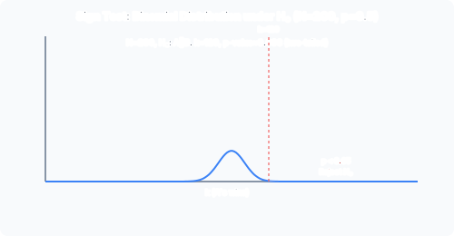
The sign test determines whether System A is significantly better than System B on a classification task. It tests the null hypothesis that both systems are equally good and any observed differences are due to chance.

Setup

• H0 (null hypothesis): Systems A and B are identical; differences are due to chance.
• H1 (alternative): System A is better than System B (one-tailed) or systems differ (two-tailed).
• Compare item by item: for each document, note whether A wins, B wins, or they tie.

The MLRD Tie Rule (CRITICAL)

Standard statistics textbooks say to discard ties. For classification tasks, this is wrong. Discarding ties reduces $N$, inflating the test statistic and causing a Type 1 error (falsely claiming significance).

The MLRD rule: distribute ties evenly. Let $d$ = number of ties. Add $d/2$ to $k$ (A’s wins) and $d/2$ to $(N - k)$ (B’s wins). Round $k$ up at the end. $N$ remains unchanged.

Test Statistic

Under H0, each item is equally likely to favour A or B (ignoring ties). Test statistic:

$X \sim \text{Binomial}(N, p = 0.5)$

$k = \text{items where A beats B} + \frac{d}{2}$

• One-tailed p-value: $P(X \geq k \mid N, p=0.5)$
• Two-tailed p-value: $2 \times P(X \geq k \mid N, p=0.5)$

If $p \leq 0.05$: reject H0; A is significantly better. If $p > 0.05$: inconclusive; cannot claim A is better.

Full Worked Example

200 documents are classified by both System A and System B:

• A wins on 110 documents
• B wins on 70 documents
• Ties on 20 documents

Step 1 — Apply the tie rule: $k = 110 + 20/2 = 110 + 10 = 120$ $N = 200$ (unchanged) $(N - k) = 200 - 120 = 80$

Step 2 — Two-tailed test: We test whether A differs from B (in either direction). Under H0, $X \sim \text{Binomial}(200, 0.5)$.

$p = 2 \times P(X \geq 120 \mid N=200, p=0.5)$

For a binomial with $N=200$, $p=0.5$, the mean is $Np = 100$ and variance is $Np(1-p) = 50$. We can approximate using the normal distribution:

$z = \frac{k - Np}{\sqrt{Np(1-p)}} = \frac{120 - 100}{\sqrt{50}} = \frac{20}{7.071} \approx 2.828$

From standard normal tables: $P(Z \geq 2.828) \approx 0.0023$.

Two-tailed $p = 2 \times 0.0023 = 0.0046$.

Step 3 — Conclusion: $p = 0.0046 < 0.05$. Reject H0. System A is significantly better than System B.

If we had discarded ties (wrong): $N = 180$, $k = 110$, $z = (110 - 90)/\sqrt{45} = 20/6.708 \approx 2.981$, giving a smaller p-value. This inflates the apparent significance, risking a false claim.

Why Not Discard Ties?

Discarding ties reduces $N$ from 200 to 180. The test statistic $z = (k - N/2)/\sqrt{N/4}$ increases because the denominator $\sqrt{N}$ shrinks while the numerator stays similar. This makes the test more likely to reject H0 even when A and B are truly identical (Type 1 error). The MLRD rule keeps $N$ fixed and distributes ties as half-wins, which is more conservative and honest.

Summary

Step	Action
1	Count A wins, B wins, ties
2	$k = \text{A wins} + (\text{ties}/2)$, round up
3	$N$ unchanged
4	Compute $p = P(X \geq k \mid \text{Binomial}(N, 0.5))$
5	If two-tailed, multiply by 2
6	Compare to $\alpha = 0.05$

Past paper questions: y2023p3q8 (evaluation methods)