Zipf's Law

The Law

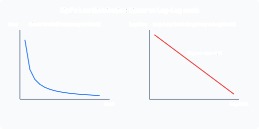
Word frequency is inversely proportional to frequency rank. A small number of words are very frequent; a huge number of words are rare.

Basic form:

$f_w \propto \frac{1}{r_w}$

where $f_w$ is the frequency of word $w$ and $r_w$ is its rank (1 = most frequent).

General form:

$f_w \approx \frac{k}{(r_w + \beta)^\alpha}$

• $f_w$: frequency of word $w$ in the corpus
• $r_w$: frequency rank (1 = most frequent)
• $\alpha$: exponent (~1.0 for English, ~1.3 for German)
• $k$, $\beta$: language-specific constants

Log-Log Estimation

Taking logs of the basic form:

$\log(f_w) = \log(k) - \alpha \cdot \log(r_w)$

Plotting $\log(\text{frequency})$ against $\log(\text{rank})$ gives a straight line:

• Slope = $-\alpha$ (estimate $\alpha$ from the slope)
• Y-intercept = $\log(k)$ (estimate $k = e^{\text{intercept}}$)

Estimate $\alpha$ and $k$ by fitting a least-squares regression to the log-log plot.

The Long Tail

In a typical English corpus:

• The top 10 words (the, of, and, to, a, …) account for ~25% of all tokens.
• The top 100 words account for ~50%.
• Thousands of words appear only once (hapax legomena).
• The tail is very long: a huge number of word types each appear very few times.

Consequence for Classification

The long tail means that even a large training corpus misses many word types. Any new document is likely to contain words never seen during training. For a Naive Bayes classifier without smoothing:

$P(w \mid c) = \frac{\text{count}(w, c)}{\sum_{w'} \text{count}(w', c)} = 0 \quad \text{for any unseen } w$

A single unseen word makes the entire product $P(c) \times \prod P(w_i \mid c)$ equal to zero. The classifier breaks.

This is why Laplace smoothing is not optional — Zipf’s Law guarantees that unseen words are ubiquitous, not rare exceptions.

Worked Example

Consider “the” (rank 1, frequency ~70,000 per million words) and “antidisestablishmentarianism” (estimated rank ~50,000, frequency < 1 per million). The ratio is roughly 70,000:1, consistent with $\alpha \approx 1$.

If a test document uses a rare word not in the training data (and there are tens of thousands of such words in the long tail), the unsmoothed NB classifier assigns probability zero to every class. Smoothing fixes this by shifting a small amount of probability mass from frequent words to the long tail.

Summary

Aspect	Detail
Basic Zipf	$f_w \propto 1/r_w$
General form	$f_w = k / (r_w + \beta)^\alpha$
$\alpha$ (English)	~1.0
$\alpha$ (German)	~1.3
Estimation	Least-squares on log-log plot
Consequence for NB	Long tail of unseen words kills unsmoothed classifier

Past paper questions: y2024p3q7 (feature engineering sub-question)