Degree and Clustering Coefficient

Degree

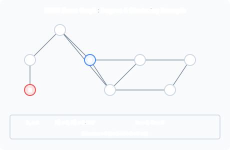
Definition: $k_i$ = number of edges incident to node $i$. For undirected graphs, this is simply the count of neighbours. For directed graphs, separate into in-degree ($k_i^{\text{in}}$) and out-degree ($k_i^{\text{out}}$).

Interpretation: the simplest measure of a node’s local connectivity or “importance”. Nodes with high degree are local hubs. Degree alone does not tell you whether the neighbours are connected to each other — that requires the clustering coefficient.

Local Clustering Coefficient

Definition: the fraction of a node’s neighbours that are connected to each other.

$C_i = \frac{2e_i}{k_i(k_i - 1)}$

where:

• $e_i$ = number of edges between the neighbours of node $i$.
• $k_i(k_i - 1)/2$ = total number of possible edges between $k_i$ neighbours (the number of unique unordered pairs of neighbours).

Interpretation:

• $C_i = 0$: none of $i$‘s neighbours are connected to each other. $i$ is like the centre of a star.
• $C_i = 1$: all of $i$‘s neighbours form a complete subgraph (a clique). Every pair of neighbours is directly connected.
• For a node with $k_i < 2$, the denominator is 0, so $C_i$ is undefined. By convention, $C_i = 0$ for such nodes (or they are excluded from the average).

What it measures: the degree of triadic closure around node $i$. High $C_i$ means $i$‘s friends are also friends with each other — characteristic of close-knit social groups. Low $C_i$ means $i$ connects otherwise disconnected people — characteristic of brokers or connectors.

Worked Example: 2025 Q8 Graph

Graph edges: A–B, A–E, B–C, B–F, C–D, D–F, D–H, F–G, G–H, C–F.

Node A

$k_A = 2$ (neighbours: B and E).

Edges between neighbours $\{B, E\}$: is there a B–E edge? No.

$e_A = 0 \qquad C_A = \frac{2 \cdot 0}{2 \cdot 1} = 0$

A’s neighbours are not connected to each other. A is like the centre of a “V” shape spanning B and E.

Node C

$k_C = 3$ (neighbours: B, D, F).

Edges among $\{B, D, F\}$:

• B–F: yes (edge exists).
• B–D: no (no direct edge).
• D–F: yes (edge exists).

$e_C = 2 \qquad \text{possible pairs} = \frac{3 \cdot 2}{2} = 3 \qquad C_C = \frac{2 \cdot 2}{3 \cdot 2} = \frac{4}{6} = 0.667$

C’s neighbours are well-connected: 2 out of 3 possible edges exist. Only the B–D edge is missing. This reflects that C sits within a fairly tight social cluster.

Node H

$k_H = 2$ (neighbours: D and G).

Edges between neighbours $\{D, G\}$: is there a D–G edge? No (D connects to H and F; G connects to H and F; D and G are not directly connected).

$e_H = 0 \qquad C_H = \frac{2 \cdot 0}{2 \cdot 1} = 0$

H is at the end of the D–H–G branch with no closure between its two neighbours.

Measuring Overall Clustering

To measure the degree to which nodes form clusters in a network, compute the average local clustering coefficient over all nodes with $k_i \geq 2$:

$\bar{C} = \frac{1}{|\{i : k_i \geq 2\}|} \sum_{i: k_i \geq 2} C_i$

There are other measures (global clustering coefficient, transitivity ratio), but the local clustering coefficient is the one required for MLRD exam answers. Social networks have high $\bar{C}$ (often 0.1–0.5); technological and information networks have low $\bar{C}$.

Summary

Measure	Formula	Node A	Node C	Node H
Degree $k_i$	Count of incident edges	2	3	2
$e_i$	Edges between neighbours	0	2	0
Possible pairs	$k_i(k_i-1)/2$	1	3	1
$C_i$	$2e_i / (k_i(k_i-1))$	0	$0.667$	0
Interpretation	—	Star centre	Partial clique	Leaf

Past paper questions: y2025p3q8