Hidden Markov Models: Definition

Motivation

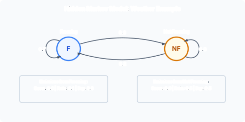
Naive Bayes treats every observation independently: word order does not matter. But many real-world problems involve sequences where items depend on their neighbours: speech, weather patterns, financial time series, biological sequences (DNA, proteins). Hidden Markov Models explicitly model these temporal dependencies through a two-level structure: hidden states that evolve over time and visible observations emitted by those states.

Formal Definition: $\mu = (S, V, A, B, \pi)$

An HMM models a system where we observe outputs (emissions) but cannot directly observe the underlying process (hidden states). The model is fully specified by five components:

Symbol	Name	Description
$S$	Hidden States	The unobservable states: $S = {s_1, s_2, \ldots, s_{
$V$	Observations	The observable emissions: $V = {v_1, v_2, \ldots, v_{
$A$	Transition Matrix	$a_{ij} = P(q_t = s_j \mid q_{t-1} = s_i)$ — row $i$, column $j$
$B$	Emission Matrix	$b_i(v_k) = P(o_t = v_k \mid q_t = s_i)$ — row $i$, column $k$
$\pi$	Initial Distribution	$\pi_j = P(q_1 = s_j)$ — probability of starting in state $j$

Each row of $A$ sums to 1. Each row of $B$ sums to 1. $\sum_j \pi_j = 1$.

Concrete Example: Weather HMM

This is the 2024 Q8 HMM. Hidden states: $S = \{\text{Freezing}(F), \text{NotFreezing}(NF)\}$ (air temperature, unobservable without a thermometer). Observations: $V = \{\text{Snow}(S), \text{Rain}(R), \text{Dry}(D)\}$ (visible weather).

Transition matrix $A$ — models how temperature changes month to month:

$q_{t-1}$ / $q_t$	$F$	$NF$
$F$	$P(F \mid F)$	$P(NF \mid F)$
$NF$	$P(F \mid NF)$	$P(NF \mid NF)$

Emission matrix $B$ — models the weather given the temperature:

$q_t$ / $o_t$	$S$	$R$	$D$
$F$	$P(S \mid F)$	$P(R \mid F)$	$P(D \mid F)$
$NF$	$P(S \mid NF)$	$P(R \mid NF)$	$P(D \mid NF)$

Note: Snow requires freezing temperatures ($P(S \mid NF) \approx 0$). Rain implies above-freezing ($P(R \mid F) \approx 0$). Dry is possible in either state.

Initial distribution $\pi$: $\pi = [P(q_1 = F),\; P(q_1 = NF)]$.

What Makes HMMs Different from Naive Bayes

Naive Bayes: $P(c \mid d) \propto P(c) \prod_i P(w_i \mid c)$ — each word contributes independently. Word order does not matter. “The dog bit the man” and “The man bit the dog” are identical to NB.

HMMs model the dependence between consecutive items through the transition matrix $A$. The hidden state at time $t$ depends on the hidden state at $t-1$. The observation at time $t$ depends on the state at $t$. This sequential structure makes HMMs suitable for any data where context matters: part-of-speech tagging, speech recognition, activity recognition, financial regime detection.

Dual-Tape Training Data

Training requires fully labelled sequences: both the hidden state and the observation at every timestep must be known. This is called dual-tape data. Example:

Timestep	1	2	3	4	5	6	7
State ($q_t$)	L	M	H	H	H	M	M
Observation ($o_t$)	+	++	++	+++	++	++	+

From this we count transitions and emissions to estimate $A$ and $B$.

Summary

Component	Formula	Meaning
$S$	—	Set of hidden states (size $
$V$	—	Set of observable symbols (size $
$a_{ij}$	$P(q_t = s_j \mid q_{t-1} = s_i)$	Transition probability
$b_i(v_k)$	$P(o_t = v_k \mid q_t = s_i)$	Emission probability
$\pi_j$	$P(q_1 = s_j)$	Initial state probability
Rows sum to 1	$\sum_j a_{ij} = 1$, $\sum_k b_i(v_k) = 1$	Valid probability distributions

Past paper questions: y2024p3q8, y2025p3q9