Skip to content
Back to Modules
Part IA Lent Term

Algorithms II

Algorithms Graphs Shortest-Paths Maximum-Flow Minimum-Spanning-Trees Amortized-Analysis Heaps Disjoint-Sets Geometric-Algorithms Part IA Lent Term
  • Graphs and Representations

    Graph terminology, adjacency matrices versus adjacency lists, and special graph classes (DAGs, bipartite, trees)

    • Graph Terminology

      Vertices and Edges

      A graph G=(V,E)G = (V, E) consists of a set of vertices (nodes) VV and a set of edges (arcs) EV×VE \subseteq V \times V. We only consider finite graphs where V|V| and E|E| are finite.

      Directed graphs have ordered pairs (u,v)E(u, v) \in E, drawn with an arrow from uu (tail) to vv (head). uu is the source and vv the destination of the edge. Undirected graphs have unordered pairs (or the edge relation is symmetric); an undirected edge {u,v}\{u, v\} is conceptually equivalent to having both directed edges (u,v)(u, v) and (v,u)(v, u).

      A simple graph has no self-loops (edges from a vertex to itself: (v,v)(v, v)) and no parallel edges (multiple edges between the same ordered pair of vertices). Unless stated otherwise, the syllabus deals with simple graphs. A multigraph allows parallel edges; a pseudograph also allows self-loops.

      A weighted graph associates a real number with each edge via a function w:ERw: E \to \mathbb{R}. Weights represent cost, distance, time, capacity, or any additive metric. Unweighted graphs can be considered as having unit weight on every edge.

      Degree

      The degree deg(v)\deg(v) of a vertex in an undirected graph is the number of edges incident at that vertex. In directed graphs:

      • In-degree deg(v)\deg^{-}(v): number of edges entering vv.
      • Out-degree deg+(v)\deg^{+}(v): number of edges leaving vv.

      Handshaking lemma: For an undirected graph, vVdeg(v)=2E\sum_{v \in V} \deg(v) = 2|E|. For directed graphs, deg(v)=deg+(v)=E\sum \deg^{-}(v) = \sum \deg^{+}(v) = |E|. A corollary: the number of odd-degree vertices in any undirected graph is always even.

      Paths, Walks, and Cycles

      A walk is any sequence of vertices where consecutive pairs are edges. A trail is a walk with no repeated edges. A path is a walk with no repeated vertices (except possibly the first/last). A simple path has no repeated vertices at all. The length of an unweighted path is the number of edges traversed (k1k-1 for kk vertices). For weighted graphs, the path length is the sum of edge weights along the path.

      A cycle (or circuit) is a path of length at least 1 that starts and ends at the same vertex with no other vertex repeated. A graph with no cycles is acyclic.

      Connectivity

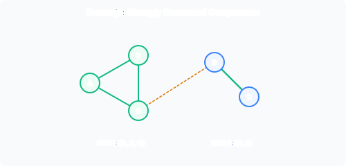
      An undirected graph is connected if there exists a path between every pair of vertices. A connected component is a maximal connected subgraph. The components partition the vertex set.

      For directed graphs, we distinguish:

      • Weak connectivity: the underlying undirected graph (ignoring edge directions) is connected.
      • Strong connectivity: for every ordered pair (u,v)(u, v), there is a directed path from uu to vv.

      Subgraphs

      • Subgraph: G=(V,E)G' = (V', E') with VVV' \subseteq V and EEE' \subseteq E.
      • Induced subgraph: select VVV' \subseteq V and include all edges from EE whose both endpoints are in VV'.
      • Spanning subgraph: V=VV' = V (contains all vertices, subset of edges).

      Trees and Forests

      A free tree (or simply tree) is a connected, acyclic undirected graph. Equivalent characterisations for a graph with nn vertices:

      1. Connected and has exactly n1n-1 edges.
      2. Acyclic and has exactly n1n-1 edges.
      3. Any two vertices are connected by exactly one simple path.
      4. Connected, and removing any edge disconnects the graph (minimally connected).
      5. Acyclic, and adding any edge creates exactly one cycle (maximally acyclic).

      A forest is an acyclic undirected graph (a collection of disjoint trees). A forest with cc components has ncn-c edges.

      Density

      ClassificationEdge countExample
      SparseE=O(V)\lvert E \rvert = O(\lvert V \rvert)Road network, planar graph
      DenseE=Θ(V2)\lvert E \rvert = \Theta(\lvert V \rvert^2)Complete graph KnK_n

      A complete graph has E=(n2)=n(n1)2|E| = \binom{n}{2} = \frac{n(n-1)}{2}. Most real-world graphs are sparse.

      Example

      Consider a road network: Cambridge (C), Oxford (O), London (L), York (Y). Roads: C—O (80), C—L (55), L—Y (210).

      • V={C,O,L,Y}V = \{C, O, L, Y\}, V=4|V|=4. E={(C,O),(C,L),(L,Y)}E = \{(C,O), (C,L), (L,Y)\}, E=3|E|=3.
      • deg(C)=2\deg(C)=2, deg(O)=1\deg(O)=1, deg(L)=2\deg(L)=2, deg(Y)=1\deg(Y)=1.
      • The graph is connected but not complete (missing 3 possible edges).
      • E=3=O(4)|E| = 3 = O(4), so it is sparse.

      Summary

      TermDefinition
      GraphG=(V,E)G = (V, E)
      DirectedOrdered pairs (u,v)(u, v)
      UndirectedUnordered pairs {u,v}\{u, v\}
      Simple graphNo self-loops, no parallel edges
      Weighted graphw:ERw: E \to \mathbb{R}
      DegreeIncident edges per vertex
      PathSequence of distinct vertices connected by edges
      CycleClosed path, no vertex repeated except start=end
      ConnectedPath exists between every pair
      TreeConnected and acyclic; E=V1\lvert E \rvert = \lvert V \rvert - 1
      SparseE=O(V)\lvert E \rvert = O(\lvert V \rvert)
      DenseE=Θ(V2)\lvert E \rvert = \Theta(\lvert V \rvert^2)

      Past paper questions: y2025p1q9 (connected components, BFS on adjacency matrix).
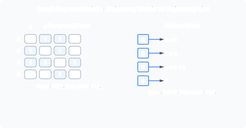
    • Adjacency Matrix versus Adjacency Lists

      Two Standard Representations

      There are two fundamental ways to store a graph in memory. The choice of representation directly affects the asymptotic running time of graph algorithms, so understanding the trade-offs is critical for both implementation decisions and exam questions.

      Adjacency matrix vs adjacency list representations

      Adjacency Matrix

      An adjacency matrix is a V×V|V| \times |V| matrix MM. For unweighted graphs:

      M[u][v]={1if (u,v)E0otherwiseM[u][v] = \begin{cases} 1 & \text{if } (u, v) \in E \\ 0 & \text{otherwise} \end{cases}

      For weighted graphs, M[u][v]M[u][v] stores the edge weight (and typically \infty, 0, or some sentinel for absent edges). For undirected graphs, the matrix is symmetric: M[u][v]=M[v][u]M[u][v] = M[v][u]. This means only the upper or lower triangle needs to be stored explicitly, roughly halving the memory. For unweighted graphs, each entry can be a single bit.

      Space: Θ(V2)\Theta(|V|^2) regardless of the number of edges. Even a graph with zero edges allocates a full matrix.

      Key operations:

      • Test if (u,v)E(u, v) \in E: O(1)O(1) — single array lookup.
      • List all neighbours of vertex uu: Θ(V)\Theta(|V|) — must scan the entire row uu.
      • Iterate over all edges: Θ(V2)\Theta(|V|^2) — must visit every matrix cell.
      • Add or remove an edge: O(1)O(1) — set or clear a cell.

      Adjacency Lists

      An array AA of length V|V|, where A[u]A[u] points to a linked list or dynamic array containing all vv such that (u,v)E(u, v) \in E. For weighted graphs, each list entry stores (v,w(u,v))(v, w(u,v)).

      Space: Θ(V+E)\Theta(|V| + |E|). Each directed edge contributes one list entry. For undirected graphs, each edge appears in two lists, so space is Θ(V+2E)=Θ(V+E)\Theta(|V| + 2|E|) = \Theta(|V| + |E|).

      Key operations:

      • Test if (u,v)E(u, v) \in E: O(deg(u))O(\deg(u)) — sequential scan of uu‘s list. Worst case O(V)O(|V|) when deg(u)=V1\deg(u) = |V|-1.
      • List neighbours of uu: Θ(deg(u))\Theta(\deg(u)) — exactly the list length.
      • Iterate over all edges: Θ(V+E)\Theta(|V| + |E|) — visit each list head and each entry once.
      • Add edge: O(1)O(1) (prepend to list). Remove edge: O(deg(u))O(\deg(u)) (find and delete).
      • For undirected graphs, removal must be done from both endpoints’ lists: O(deg(u)+deg(v))O(\deg(u) + \deg(v)).

      Worked Example

      Directed weighted graph: V={1,2,3,4}V = \{1, 2, 3, 4\}, edges (1,2)(1,2) weight 5, (1,3)(1,3) weight 2, (2,4)(2,4) weight 1.

      Matrix representation: (0520100)\begin{pmatrix} 0 & 5 & 2 & \infty \\ \infty & 0 & \infty & 1 \\ \infty & \infty & 0 & \infty \\ \infty & \infty & \infty & 0 \end{pmatrix}

      Adjacency list representation:

      • A[1](2,5)(3,2)A[1] \to (2,5) \to (3,2)
      • A[2](4,1)A[2] \to (4,1)
      • A[3]A[3] \to \emptyset
      • A[4]A[4] \to \emptyset

      Space analysis: matrix uses 4×4=164 \times 4 = 16 entries. Lists use 3 list entries + 4 array slot pointers = 7 entries. For this sparse graph (E=3|E|=3 of a possible 12), lists are significantly more compact.

      Trade-off Summary

      CriterionAdjacency MatrixAdjacency Lists
      SpaceΘ(V2)\Theta(V^2)Θ(V+E)\Theta(V + E)
      Edge query (u,v)(u,v)O(1)O(1)O(deg(u))O(V)O(\deg(u)) \le O(V)
      Neighbours of uuΘ(V)\Theta(V)Θ(deg(u))\Theta(\deg(u))
      All edges iterationΘ(V2)\Theta(V^2)Θ(V+E)\Theta(V + E)
      Add edgeO(1)O(1)O(1)O(1)
      Remove edgeO(1)O(1)O(deg(u)+deg(v))O(\deg(u) + \deg(v))
      Best forDense graphsSparse graphs

      Impact on Graph Algorithms

      BFS/DFS: With adjacency lists, both run in Θ(V+E)\Theta(|V| + |E|) because the inner loop visits each neighbour exactly once. With an adjacency matrix, the inner loop must scan all V|V| columns for each dequeued/extracted vertex, costing Θ(V)\Theta(|V|) per vertex. Total: O(V2)O(|V|^2) regardless of edge count.

      Exam point (y2025p1q9): Tight bounds for BFS with adjacency matrix are Ω(V2)\Omega(|V|^2) and O(V2)O(|V|^2); with lists, Ω(V+E)\Omega(|V|+|E|) and O(V+E)O(|V|+|E|).

      Dijkstra: With binary heap and adjacency lists: O((V+E)logV)O((|V|+|E|)\log |V|). With matrix: neighbour iteration becomes Θ(V)\Theta(|V|) per vertex, and using a simple array instead of heap gives O(V2)O(|V|^2), which can be faster than O(V2logV)O(|V|^2 \log |V|) for dense graphs due to lower constants.

      Floyd-Warshall: Inherently uses a matrix (the distance matrix itself), running in Θ(V3)\Theta(|V|^3). Johnson’s algorithm relies on adjacency lists for sparsely efficient Dijkstra calls.

      Summary

      PropertyMatrixLists
      SpaceΘ(V2)\Theta(V^2)Θ(V+E)\Theta(V+E)
      Edge testO(1)O(1)O(V)O(V) worst
      Neighbour listingΘ(V)\Theta(V)Θ(deg(v))\Theta(\deg(v))
      BFS/DFS timeO(V2)O(V^2)Θ(V+E)\Theta(V+E)
      Use whenE=Θ(V2)E = \Theta(V^2)E=O(V)E = O(V)

      Past paper questions: y2025p1q9(a)(i) (BFS complexity bounds with adjacency matrix).
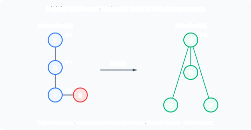
    • Königsberg Bridges and Eulerian Paths

      The Seven Bridges Problem

      In 1736, Leonhard Euler considered the city of Königsberg (now Kaliningrad), which straddled the Pregel River. Seven bridges connected four landmasses (two riverbanks and two islands). The puzzle: could a citizen walk through the city, crossing every bridge exactly once, and return to the starting point?

      Euler’s key insight was to abstract away geography: landmasses become vertices, bridges become edges. This produced the first formal graph-theoretic argument in history. Euler proved no such walk exists: the four landmasses have degrees 3, 3, 3, and 5 (all odd), making an Eulerian circuit impossible. Beyond solving a puzzle, Euler established graph theory as a mathematical discipline.

      Eulerian Paths and Circuits

      An Eulerian path (or trail) visits every edge in the graph exactly once; vertices may be revisited. An Eulerian circuit (or tour) is an Eulerian path that starts and ends at the same vertex.

      Theorem (undirected graphs): A connected, undirected graph has an Eulerian circuit iff every vertex has even degree. It has an Eulerian path but not a circuit iff exactly zero or two vertices have odd degree; if two, the path must start at one odd-degree vertex and end at the other. If more than two vertices have odd degree, no Eulerian path exists.

      Directed version: An Eulerian circuit exists iff every vertex has in-degree equal to out-degree and the graph is strongly connected (ignoring isolated vertices). An Eulerian path (start ≠ end) exists iff exactly one vertex has out-degree == in-degree +1+ 1 (start), one vertex has in-degree == out-degree +1+ 1 (end), and all other vertices have in-degree == out-degree.

      Proof Sketch: Necessity

      In an Eulerian circuit, every time the walk enters a vertex (except the start/end) it must also leave via a different edge. Thus each visit consumes two incident edges, one for entry and one for exit. For the circuit to cover every edge exactly once, each vertex must have an even number of incident edges in total. If the walk is a path from aa to bb (aba \neq b), vertex aa has one more exit than entry, bb has one more entry than exit, and all others are balanced, giving exactly two odd-degree vertices.

      Sufficiency: If all degrees are even, construct the circuit by greedily following unused edges from the current vertex. When stuck (returned to start), you have a closed trail. Remove those edges; the remaining subgraph still has all even degrees. Recursively find circuits in each connected component and splice them into the main circuit at shared vertices. This construction is called Hierholzer’s algorithm and runs in Θ(V+E)\Theta(|V| + |E|).

      Worked Example 1: Königsberg

      Landmasses: two riverbanks (north, south), two islands (Kneiphof, Lomse). Bridges: 5 connect to Kneiphof, 3 to the north bank, 3 to the south bank, 3 to Lomse. In the graph, every vertex has odd degree (3, 3, 3, 5). Since all are odd, Euler’s theorem says no Eulerian circuit or path exists. The problem is impossible.

      Worked Example 2: Modified Bridge Network

      Suppose one bridge is added between the two riverbanks, making degrees: 4, 4, 3, 3. Now exactly two vertices have odd degree (3). An Eulerian path exists, starting at one odd-degree vertex and ending at the other.

      Worked Example 3: Simple Abstract Graph

      Graph with vertices {A,B,C,D}\{A,B,C,D\} and edges: {A,B},{A,C},{B,C},{B,D},{C,D}\{A,B\}, \{A,C\}, \{B,C\}, \{B,D\}, \{C,D\} (five edges). Degrees: deg(A)=2\deg(A)=2, deg(B)=3\deg(B)=3, deg(C)=3\deg(C)=3, deg(D)=2\deg(D)=2. Exactly two odd-degree vertices (B and C). Eulerian path: BACDBCB \to A \to C \to D \to B \to C. No circuit exists (B and C are odd).

      Graph Invariants

      The parity of vertex degrees (the count of odd-degree vertices) is a graph invariant preserved under isomorphism. In Königsberg, the parity multiset is {3,3,3,5}\{3,3,3,5\}, all odd; no isomorphic graph with all even degrees can exist. This is an early example of an invariant proof: properties preserved by isomorphism can be used to prove non-isomorphism.

      Modern Applications

      • Chinese Postman Problem: Find the shortest closed walk covering every edge at least once. Solved by identifying odd-degree vertices, computing a minimum-weight perfect matching among them (to determine which edges to duplicate), then finding an Eulerian circuit. Runs in O(V3)O(|V|^3) due to the matching step. Applications in postal delivery, street sweeping, and gritting routes.
      • DNA fragment assembly (de Bruijn graphs): Sequencing produces short overlapping reads (k-mers). A de Bruijn graph is built where edges represent k-mers and vertices represent (k-1)-mer overlaps. An Eulerian path through this graph reconstructs the original genome sequence. This scales much better than Hamiltonian-path alternatives for large genomes.
      • PCB testing: Test probes must traverse every trace on a circuit board exactly once; this is an Eulerian path problem.
      • Snow plough routing: After a snowfall, every street must be ploughed; the problem reduces to Eulerian circuit construction on a multigraph (multiple lanes per road).

      Key Distinction

      • Eulerian: visits every edge exactly once. Solvable in Θ(V+E)\Theta(|V| + |E|).
      • Hamiltonian: visits every vertex exactly once. NP-complete in general; no efficient algorithm is known.

      Do not confuse these two in exam answers.

      Summary

      ConceptCondition
      Eulerian circuit (undirected)All vertices have even degree
      Eulerian path (start ≠ end)Exactly 0 or 2 odd-degree vertices
      No Eulerian walk4\ge 4 odd-degree vertices
      Directed Eulerian circuitin-degree = out-degree for all vertices
      Existence checkΘ(V)\Theta(V) (count degrees)
      Construction (Hierholzer)Θ(V+E)\Theta(V+E)
      Chinese PostmanO(V3)O(V^3) (matching on odd-degree vertices)

      Past paper questions: Not a heavily examined standalone topic, but graph invariants and parity arguments appear in proofs. Connected components and BFS are related exam topics (y2025p1q9).

    • Special Graph Classes

      Directed Acyclic Graphs (DAGs)

      A DAG is a directed graph containing no directed cycles. Many real-world dependency structures are naturally acyclic: course prerequisites, build system targets (make), version histories.

      Existence of sources and sinks: Every DAG has at least one source (in-degree 0) and at least one sink (out-degree 0). Proof: pick any vertex and follow incoming edges backward. Since there are no cycles and the graph is finite, this walk must terminate at a source. Symmetrically, following outgoing edges forward reaches a sink. This property is used in the source-removal topological sort algorithm.

      Topological ordering: A linear ordering exists such that all edges go left to right iff the graph is a DAG. See topological sort for the full algorithm.

      SSSP on DAGs: Relax edges in topological order. Correctness: when vertex uu is processed, all incoming paths to uu have already been considered because all predecessors appear earlier in the topological order. Thus one pass suffices. Running time: Θ(V+E)\Theta(|V| + |E|), even with negative edge weights (provided no cycles exist, which they cannot in a DAG). This is the fastest SSSP algorithm amongst those covered.

      Longest path on DAGs: By negating all edge weights, or replacing min\min with max\max during relaxation, the longest path can also be found in Θ(V+E)\Theta(|V| + |E|). For general graphs, the longest path problem is NP-hard; DAGs are a notable exception.

      Bipartite Graphs

      A graph is bipartite if its vertex set can be partitioned into two disjoint sets LL and RR such that every edge has one endpoint in each set. No edges exist within LL or within RR.

      Characterisation: An undirected graph is bipartite iff it contains no cycle of odd length. A graph with a triangle (K3K_3) is never bipartite; a tree is always bipartite.

      Testing bipartiteness (BFS-based algorithm):

      1. Pick any unvisited vertex, colour it BLACK.
      2. Run BFS from it. Colour each vertex at distance dd: BLACK if dd is even, RED if dd is odd (alternating by parity).
      3. Scan all edges. If any edge connects two vertices of the same colour, an odd cycle exists — the graph is not bipartite.
      4. Repeat for each connected component until all vertices are processed.

      Both colouring and conflict checking run in O(V+E)O(|V|+|E|), so the full test is Θ(V+E)\Theta(|V|+|E|). BFS’s distance-level property guarantees the alternating colour assignment is correct: vertices at the same BFS level cannot be adjacent in a bipartite graph.

      Worked example: 4-cycle: V={1,2,3,4}V = \{1,2,3,4\}, E={{1,2},{2,3},{3,4},{4,1}}E = \{\{1,2\}, \{2,3\}, \{3,4\}, \{4,1\}\}. BFS from 1: dist(1)=0 (BLACK), dist(2)=dist(4)=1 (RED), dist(3)=2 (BLACK). No conflict — bipartite with L={1,3}L=\{1,3\}, R={2,4}R=\{2,4\}.

      Worked non-example: Triangle K3K_3: V={1,2,3}V=\{1,2,3\}, E={{1,2},{2,3},{3,1}}E=\{\{1,2\},\{2,3\},\{3,1\}\}. BFS from 1: dist(1)=0 (BLACK), dist(2)=dist(3)=1 (RED). Edge {2,3}\{2,3\} connects two RED vertices — conflict, not bipartite.

      Applications: Matching problems (assigning students to rooms, workers to tasks) are modelled as bipartite graphs. Maximum bipartite matching reduces to a max-flow problem and can be solved with Ford-Fulkerson or Hopcroft-Karp.

      Complete Graphs

      The complete graph KnK_n has all (n2)\binom{n}{2} possible edges; every vertex has degree n1n-1. KnK_n is (n1)(n-1)-regular. A clique is any complete induced subgraph.

      Trees (Detailed)

      For an undirected graph on nn vertices, the following are equivalent definitions of a tree:

      1. Connected and acyclic.
      2. Connected and has exactly n1n-1 edges.
      3. Acyclic and has exactly n1n-1 edges.
      4. Between any two vertices, exactly one simple path exists.
      5. Maximally acyclic: adding any edge creates exactly one cycle.
      6. Minimally connected: removing any edge disconnects the graph.

      Every tree with n2n \ge 2 has at least two leaves (vertices of degree 1). A rooted tree designates one vertex as root; parent and child relationships emerge from distances to the root. The depth of a vertex is its distance from the root. A binary tree restricts each vertex to at most two children. Every tree is bipartite (alternate levels).

      Transpose, Complement, and Square

      • Transpose GTG^T: reverses all edges. (u,v)E    (v,u)ET(u,v) \in E \iff (v,u) \in E^T. Essential for Kosaraju’s algorithm.
      • Complement G\overline{G}: same vertices, (u,v)E(G)(u,v) \in E(\overline{G}) iff (u,v)E(G)(u,v) \notin E(G). A clique in GG is an independent set in G\overline{G}.
      • Square G2G^2: edge (u,v)(u,v) exists iff a path of length 2\le 2 connects them in GG.

      Summary

      Graph ClassKey PropertyDetection Time
      DAGNo directed cycles; 1\ge 1 source and sinkΘ(V+E)\Theta(V+E) (DFS)
      BipartiteNo odd cycles; 2-colourableΘ(V+E)\Theta(V+E) (BFS)
      Complete KnK_nAll (n2)\binom{n}{2} edges presentO(1)O(1) (check degrees)
      TreeE=V1\lvert E \rvert = \lvert V \rvert - 1, connected and acyclicΘ(V+E)\Theta(V+E) (DFS/BFS)
      ForestDisjoint union of treesΘ(V+E)\Theta(V+E)
      PropertyDAGGeneral digraph
      SSSP timeΘ(V+E)\Theta(V+E)O((V+E)logV)O((V+E)\log V) / O(VE)O(VE)
      Longest pathΘ(V+E)\Theta(V+E)NP-hard
      Topological sortAlways existsOnly if acyclic

      Past paper questions: y2026p1q10 (DAG, topological sort, transitive closure for DAGs), y2025p1q9(b)(i) (connected components labelling).

  • Graph Traversal

    Breadth-first search and its properties, depth-first search, edge classification, and topological sort

    • Breadth-First Search: Algorithm

      Overview

      Breadth-First Search (BFS) explores vertices in order of increasing distance from a source vertex ss. It uses a FIFO queue to manage the frontier. BFS discovers every vertex reachable from ss and computes the shortest-path distance (in terms of number of edges) for unweighted graphs.

      Colour Scheme

      BFS uses three colours to track vertex state:

      • White: undiscovered (initial state for all vertices).
      • Grey: discovered but not yet fully explored (currently in or awaiting processing from the queue).
      • Black: finished; all neighbours have been examined.

      These colours prevent enqueuing the same vertex twice — a key distinction from naive tree traversal. Without the pending/grey marker, a vertex could be enqueued multiple times, wasting memory and time.

      Pseudocode

      BFS(G, s):
        for each v in G.V:
          v.colour = WHITE
          v.d = ∞             // distance from source
          v.π = NIL            // predecessor
        s.colour = GREY
        s.d = 0
        s.π = NIL
        Q = new Queue()
        ENQUEUE(Q, s)
        while Q not empty:
          u = DEQUEUE(Q)
          for each v in G.Adj[u]:
            if v.colour == WHITE:
              v.colour = GREY
              v.d = u.d + 1
              v.π = u
              ENQUEUE(Q, v)
          u.colour = BLACK

      How It Works

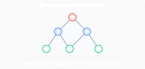
      BFS traversal: frontier expands level by level from source vertex

      The queue stores the frontier: vertices discovered but whose neighbours have not yet been examined. Because vertices are enqueued in order of discovery (and thus by distance), BFS explores distance kk vertices before any distance k+1k+1 vertex.

      The predecessor array π\pi implicitly defines a breadth-first tree: the edges (v.π,v)(v.\pi, v) for all vv with v.πNILv.\pi \neq \text{NIL} form a tree rooted at ss. Following π\pi pointers backwards from any vertex reconstructs a shortest path to ss.

      Worked Example

      Consider an undirected graph with V={A,B,C,D,E}V = \{A,B,C,D,E\} and edges: ABA-B, ACA-C, BDB-D, CDC-D, DED-E. Source s=As = A.

      StepQueued(A)d(B)d(C)d(D)d(E)
      Init[A]0
      Deq A[B,C]011
      Deq B[C,D]0112
      Deq C[D]0112
      Deq D[E]01123
      Deq E[]01123

      Predecessor tree: π(B)=A\pi(B)=A, π(C)=A\pi(C)=A, π(D)=B\pi(D)=B (first visit), π(E)=D\pi(E)=D. Shortest path A→E: E→D→B→A (reverse gives A-B-D-E, distance 3).

      Complexity Analysis

      With adjacency lists: the initialisation loop and the outer while loop touch each vertex once (Θ(V)\Theta(|V|)). The inner for loop traverses each edge’s adjacency list entry at most once (Θ(E)\Theta(|E|) for directed, at most 2E2|E| for undirected). Total: Θ(V+E)\Theta(|V| + |E|).

      With adjacency matrix: the inner loop must scan all V|V| columns for each dequeued vertex to check if an edge exists. This costs Θ(V)\Theta(|V|) per vertex, giving O(V2)O(|V|^2) overall. For sparse graphs this is significantly worse.

      Key Point: Duplicate Enqueue Prevention

      A naive implementation that checks only marked at dequeue time (not at enqueue) can insert the same vertex into the queue multiple times. The GREY/pending flag prevents this: once a vertex is discovered, its colour changes to grey immediately, so subsequent edges to it are ignored.

      Summary

      AspectDetail
      Data structureFIFO queue
      Colour schemeWhite → Grey → Black
      Distance metricEdge count (unweighted)
      Outputd[v]d[v] (shortest distance), π[v]\pi[v] (predecessor)
      Time (adj. lists)Θ(V+E)\Theta(V+E)
      Time (adj. matrix)Θ(V2)\Theta(V^2)
      SpaceΘ(V)\Theta(V) (queue) + Θ(V+E)\Theta(V+E) (graph)

      Past paper questions: y2025p1q9(a)(i) (BFS time bounds with adjacency matrix).

    • BFS: Correctness and Properties

      What We Need to Prove

      When BFS terminates, for every vertex vv reachable from source ss, the value v.dv.d equals the true shortest-path distance δ(s,v)\delta(s, v) (the minimum number of edges on any path from ss to vv). For unreachable vertices, v.d=δ(s,v)=v.d = \delta(s, v) = \infty. Additionally, following predecessor π\pi pointers backwards from any vertex reconstructs a shortest path to ss.

      The proof proceeds through three lemmas, culminating in a contradiction argument that no vertex can be the “first” to receive a wrong distance.

      Lemma 1: Upper Bound on Neighbour Distance

      If (u,v)E(u, v) \in E, then δ(s,v)δ(s,u)+1\delta(s, v) \le \delta(s, u) + 1.

      Proof: If uu is unreachable from ss, then δ(s,u)=\delta(s, u) = \infty and the inequality trivially holds. If uu is reachable, the shortest path to vv is at most the shortest path to uu plus one more edge (u,v)(u, v). It cannot be longer than that (though it could be shorter if there is a path to vv that bypasses uu). Hence the inequality.

      Lemma 2: v.dv.d Never Underestimates

      On termination, for all vVv \in V, we have v.dδ(s,v)v.d \ge \delta(s, v).

      Proof by induction on the number of enqueue operations:

      Base case: Immediately before the while loop begins: s.d=0=δ(s,s)s.d = 0 = \delta(s, s), so the hypothesis holds for ss. For all other vertices, v.d=δ(s,v)v.d = \infty \ge \delta(s, v), even if unreachable. Hypothesis holds.

      Inductive step: The while/for loops only change v.dv.d when vv is white (not pending), via the assignment v.d=u.d+1v.d = u.d + 1. By the induction hypothesis, u.dδ(s,u)u.d \ge \delta(s, u). Then: v.d=u.d+1δ(s,u)+1δ(s,v)v.d = u.d + 1 \ge \delta(s, u) + 1 \ge \delta(s, v) where the last inequality is Lemma 1. Since v.dv.d is never changed again (it becomes grey immediately), the property persists.

      This lemma says the algorithm never reports a distance too low; it may overestimate until convergence.

      Lemma 3: Queue Disciplines the Order

      Queue property ϕ\phi: If the queue is Q=v1,v2,,vxQ = v_1, v_2, \ldots, v_x (head to tail), then vx.dv1.d+1v_x.d \le v_1.d + 1 and the v.dv.d values are non-decreasing from head to tail: vi.dvi+1.dv_i.d \le v_{i+1}.d for all i=1,,x1i = 1, \ldots, x-1.

      Proof by induction on queue operations.

      • Dequeue: Removing v1v_1 leaves v2v_2 as the new head. From ϕ\phi we have vx.dv1.d+1v2.d+1v_x.d \le v_1.d + 1 \le v_2.d + 1 (since v1.dv2.dv_1.d \le v_2.d). So ϕ\phi holds after dequeue.
      • Enqueue: When vv (with v.d=u.d+1v.d = u.d + 1) is appended, we need to verify v1.dvx.dv.dv_1.d \le \cdots \le v_x.d \le v.d and v.dv1.d+1v.d \le v_1.d + 1. The first holds because vx.du.d+1v_x.d \le u.d + 1 (from ϕ\phi before dequeue, vx.dv1.d(=u.d)+1=u.d+1=v.dv_x.d \le v_1.d (= u.d) + 1 = u.d+1 = v.d). The second holds because v.d=u.d+1=v1.d+1v.d = u.d + 1 = v_1.d + 1.

      Corollary: If vertex aa is enqueued before vertex bb, then a.db.da.d \le b.d on termination. This follows from the non-decreasing property when aa and bb are simultaneously in the queue and from transitivity of \le when they are not.

      Termination: Proof by Contradiction

      Assume the algorithm errs. Let vv be the vertex with minimum δ(s,v)\delta(s, v) whose v.dδ(s,v)v.d \neq \delta(s, v). By Lemma 2, we must have v.d>δ(s,v)v.d > \delta(s, v). Also vsv \neq s (since s.d=0s.d = 0 is correct), and vv must be reachable from ss (otherwise δ(s,v)=v.d\delta(s,v) = \infty \ge v.d).

      Let uu be the immediate predecessor of vv on a true shortest path svs \leadsto v. Then δ(s,u)=δ(s,v)1\delta(s, u) = \delta(s, v) - 1. Since δ(s,u)<δ(s,v)\delta(s, u) < \delta(s, v) and vv is the minimum-δ\delta vertex with a wrong dd, we have u.d=δ(s,u)u.d = \delta(s, u). Hence: v.d>δ(s,v)=δ(s,u)+1=u.d+1v.d > \delta(s, v) = \delta(s, u) + 1 = u.d + 1

      Now consider the moment uu was dequeued from QQ. Vertex vv was in exactly one of three states:

      1. Not yet enqueued (white): The inner loop would explore the edge (u,v)(u, v) and set v.d=u.d+1v.d = u.d + 1. But we have v.d>u.d+1v.d > u.d + 1 — contradiction.
      2. In the queue (grey, pending): vv was enqueued earlier by some ww with v.d=w.d+1v.d = w.d + 1. By the corollary, w.du.dw.d \le u.d (since ww was enqueued before uu was dequeued, and uu was dequeued before vv, so wuvw \le u \le v in dequeue order). Thus v.d=w.d+1u.d+1v.d = w.d + 1 \le u.d + 1, contradicting v.d>u.d+1v.d > u.d + 1.
      3. Already dequeued (black): By the corollary, v.du.dv.d \le u.d, contradicting v.d>u.d+1v.d > u.d + 1.

      All three cases produce contradictions. Therefore no such vv exists; BFS computes correct distances for all vertices.

      Shortest-Path Tree

      The predecessor subgraph Gπ=(Vπ,Eπ)G_\pi = (V_\pi, E_\pi) where Vπ={vv.πNIL}{s}V_\pi = \{v \mid v.\pi \neq \text{NIL}\} \cup \{s\} and Eπ={(π[v],v)vV{s}}E_\pi = \{(\pi[v], v) \mid v \in V \setminus \{s\}\} forms a breadth-first tree. It is a tree because each vertex (except ss) has exactly one predecessor and no cycles exist. The unique path in GπG_\pi from ss to any reachable vv is a shortest path in GG.

      Applications

      ApplicationHow BFS solves it
      Unweighted shortest pathsv.d=δ(s,v)v.d = \delta(s,v) in edge count
      Bipartite testingColour layers alternately; check for conflicts
      Connected componentsBFS from any unvisited vertex; repeat
      Web crawlingExplore by link distance from seed
      Social network analysisDegrees of separation via BFS depth

      Summary

      PropertyStatement
      Lemma 1δ(s,v)δ(s,u)+1\delta(s,v) \le \delta(s,u) + 1 if (u,v)E(u,v) \in E
      Lemma 2v.dδ(s,v)v.d \ge \delta(s,v) at all times
      Lemma 3Queue has at most 2 consecutive dd values
      Correctnessv.d=δ(s,v)v.d = \delta(s,v) for all vv on termination
      Predecessor tree(π[v],v)(\pi[v], v) edges form a BFS tree rooted at ss

      Past paper questions: y2025p1q9(a)(i) (BFS time analysis with different representations).

    • Depth-First Search: Algorithm

      Overview

      Depth-First Search (DFS) explores as deeply as possible along each branch before backtracking. It is typically implemented recursively (the call stack acts as the LIFO stack). DFS produces a depth-first forest and assigns two integer timestamps per vertex: discovery time and finish time.

      Unlike BFS, DFS does not require a source vertex; it discovers all vertices in the graph by restarting from any unvisited vertex until all have been explored.

      Pseudocode

      DFS(G):
        for each v in G.V:
          v.colour = WHITE
          v.π = NIL
        time = 0
        for each v in G.V:
          if v.colour == WHITE:
            DFS-VISIT(G, v)
      
      DFS-VISIT(G, u):
        time = time + 1
        u.d = time              // discovery time
        u.colour = GREY
        for each v in G.Adj[u]:
          if v.colour == WHITE:
            v.π = u
            DFS-VISIT(G, v)
        u.colour = BLACK
        time = time + 1
        u.f = time              // finish time

      Timestamps

      Each vertex gets two timestamps:

      • d[v]d[v] (discovery time): when the vertex is first encountered (colour changes white → grey).
      • f[v]f[v] (finish time): when all descendants have been explored (colour changes grey → black).

      Timestamps are integers from 1 to 2V2|V|. Every vertex is discovered exactly once and finished exactly once.

      Worked Example

      Consider a directed graph: V={1,2,3,4,5,6,7,8}V = \{1,2,3,4,5,6,7,8\} with edges: 121 \to 2, 131 \to 3, 232 \to 3, 242 \to 4, 353 \to 5, 454 \to 5, 565 \to 6, 585 \to 8, 676 \to 7, 767 \to 6, 848 \to 4.

      Run DFS starting from vertex 1 (assume adjacency lists in numerical order):

      Vertex12345678
      Discover dd12345689
      Finish ff161510712111413

      The timestamps reveal ancestry: vertex 2 is a descendant of 1 because d[1]=1<d[2]=2<f[2]=15<f[1]=16d[1]=1 < d[2]=2 < f[2]=15 < f[1]=16.

      Parenthesis Theorem

      For any two vertices uu and vv, exactly one of the following holds:

      1. [d[u],f[u]][d[u], f[u]] and [d[v],f[v]][d[v], f[v]] are disjoint: neither is an ancestor of the other.
      2. [d[u],f[u]][d[u], f[u]] is fully contained within [d[v],f[v]][d[v], f[v]]: uu is a descendant of vv.
      3. [d[v],f[v]][d[v], f[v]] is fully contained within [d[u],f[u]][d[u], f[u]]: vv is a descendant of uu.

      This theorem implies: vv is a proper descendant of uu in the depth-first forest iff d[u]<d[v]<f[v]<f[u]d[u] < d[v] < f[v] < f[u].

      Complexity

      Θ(V+E)\Theta(|V| + |E|) with adjacency lists. Each vertex is discovered once, and the for loop in DFS-VISIT iterates over each adjacency list entry exactly once (or twice for undirected graphs). With an adjacency matrix, the cost becomes Θ(V2)\Theta(|V|^2).

      DFS Forest

      When DFS restarts from an unvisited vertex in the outer loop, it begins a new tree. The set of all trees forms the depth-first forest. For an undirected graph, the number of DFS trees equals the number of connected components.

      Comparison: BFS vs DFS

      PropertyBFSDFS
      Data structureQueue (FIFO)Stack (LIFO) / recursion
      Source requiredYes (ss)No
      Distance propertyShortest unweighted pathsTimestamps for ordering
      Tree typeBreadth-first treeDepth-first forest
      Edge classificationNot producedTree/back/forward/cross
      ApplicationsShortest paths, bipartite testTopological sort, SCC, cycle detection

      Summary

      AspectDetail
      Traversal orderDeepest-first, then backtracks
      ColoursWhite → Grey → Black
      Timestampsd[v]d[v] (discovery), f[v]f[v] (finish)
      Parenthesis theoremIntervals are nested or disjoint
      Time (adj. lists)Θ(V+E)\Theta(V+E)
      OutputDF forest, timestamps, edge classification

      Past paper questions: y2026p1q10 (topological sort via DFS), y2025p1q9(b)(i) (connected components).

    • DFS Edge Classification

      Four Edge Types

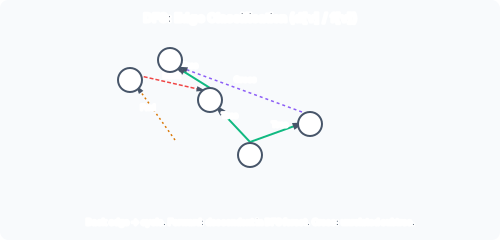
      DFS edge classification: tree, back, forward, and cross edges on a directed graph

      During DFS on a directed graph, every edge (u,v)(u, v) is classified based on the colour of the target vertex vv at the moment the edge is first explored from uu. There are four classifications:

      1. Tree edge: vv is WHITE. The edge is added to the DFS forest; vv becomes a child of uu in the depth-first tree. Discovered during: DFS-VISIT(u)v.colour == WHITE → call DFS-VISIT(v).
      2. Back edge: vv is GREY. vv is an ancestor of uu in the current DFS tree. Indicates a directed cycle exists. Example: uancestor(u)u \to \text{ancestor}(u).
      3. Forward edge: vv is BLACK and is a descendant of uu in the DFS forest (but not a direct child; direct children are tree edges). Connects a vertex to a non-child descendant.
      4. Cross edge: vv is BLACK and is neither an ancestor nor a descendant of uu. Either connects different subtrees of the same DFS tree, or connects vertices in different DFS trees entirely.

      The classification depends on DFS exploration order: the same edge might be classified differently if adjacency lists are processed in a different order.

      Timestamp-Based Characterisation

      The timestamps give precise, colour-independent criteria. For edge (u,v)(u, v):

      • Tree or forward edge iff d[u]<d[v]<f[v]<f[u]d[u] < d[v] < f[v] < f[u]. The target’s interval is nested inside the source’s. To distinguish tree from forward: for tree edges, vv was discovered via this specific edge; for forward edges, vv was discovered through a different path but is still a descendant.
      • Back edge iff d[v]d[u]<f[u]f[v]d[v] \le d[u] < f[u] \le f[v]. The target was discovered before the source and finishes after the source. This is the hallmark of cycles.
      • Cross edge iff d[v]<f[v]<d[u]<f[u]d[v] < f[v] < d[u] < f[u]. The entire interval of vv lies before the entire interval of uu.

      Properties Through an Example Walk

      Run DFS on this directed graph: 121 \to 2, 131 \to 3, 232 \to 3, 242 \to 4, 353 \to 5, 454 \to 5, 565 \to 6, 676 \to 7, 767 \to 6, 585 \to 8, 848 \to 4.

      Discovery and finish times (assuming adjacency lists in numerical order, starting from 1):

      Vertex12345678
      dd12345689
      ff161510712111413

      Classify each edge:

      • (1,2)(1,2): tree (2 white). (1,3)(1,3): forward (3 black, descendant: d[1]<d[3]<f[3]<f[1]d[1] < d[3] < f[3] < f[1], but 3 discovered via 2, not 1).
      • (2,3)(2,3): tree. (2,4)(2,4): tree.
      • (3,5)(3,5): tree.
      • (4,5)(4,5): forward (5 discovered later via 3, but is descendant of 4).
      • (5,6)(5,6): tree. (5,8)(5,8): tree.
      • (6,7)(6,7): tree.
      • (7,6)(7,6): back (6 is grey when exploring 767 \to 6; also d[6]=6d[7]=8d[6]=6 \le d[7]=8, f[6]f[6] is not assigned yet but f[7]<f[6]f[7] < f[6] — back edge).
      • (8,4)(8,4): back (4 is grey when exploring 848 \to 4; or by timestamps: d[4]=4d[8]=9d[4]=4 \le d[8]=9 and f[8]f[8] is not yet assigned before 88 finishes, but f[4]=7<f[8]=13f[4]=7 < f[8]=13 — confirms ancestor relationship).

      The presence of back edges (7,6)(7,6) and (8,4)(8,4) confirms cycles in the graph.

      Undirected Graphs

      In an undirected graph, DFS processes each edge in both directions (once from each endpoint). This restricts the possible classifications:

      • Tree edges occur when the neighbour is white.
      • Back edges occur when the neighbour is already discovered but is not the immediate parent (the vertex from which we just arrived). The edge (v,parent)(v, \text{parent}) explored in reverse is trivially a back edge under the directed definition; in the undirected context, we treat this as the reverse of the tree edge and not a cycle-indicating back edge.

      Forward and cross edges cannot occur in undirected graphs. Proof: if (u,v)(u,v) were a forward edge (descendant), then exploring from vv would encounter uu as a back edge; but the symmetric relationship means the edge would already be part of the DFS tree. Cross edges would imply exploring from uu first then from vv later, but if (u,v)E(u,v) \in E, the second exploration would encounter the other vertex immediately, making it a back edge.

      Conclusion for undirected graphs: Every edge is either a tree edge or a back edge. A back edge (to a non-parent ancestor) indicates an undirected cycle.

      Cycle Detection

      • Directed graph is a DAG iff DFS produces no back edges. Algorithm: run DFS; if any edge (u,v)(u, v) is explored with vv coloured GREY, report “contains cycle”. Time: Θ(V+E)\Theta(|V| + |E|).
      • Undirected graph has a cycle iff any non-tree back edge exists.

      This is a fundamental result: DFS provides linear-time cycle detection for both directed and undirected graphs.

      Summary

      Edge TypeTarget ColourTimestamp ConditionSignificance
      TreeWHITEd[u]<d[v]<f[v]<f[u]d[u] < d[v] < f[v] < f[u]Part of DFS forest
      BackGREYd[v]d[u]<f[u]f[v]d[v] \le d[u] < f[u] \le f[v]Indicates cycle
      ForwardBLACK, descendantd[u]<d[v]<f[v]<f[u]d[u] < d[v] < f[v] < f[u]Non-tree shortcut to descendant
      CrossBLACK, unrelatedd[v]<f[v]<d[u]<f[u]d[v] < f[v] < d[u] < f[u]Between subtrees or trees
      Graph typeAllowed edge types
      DirectedAll four types
      UndirectedTree + Back only
      ApplicationDetail
      Cycle detection in directed graphsBack edge     \iff cycle, Θ(V+E)\Theta(V+E)
      Acyclicity testNo back edges in DFS

      Past paper questions: y2026p1q10 (DAG and topological sort via DFS).

    • Topological Sort

      Definition

      A topological ordering of a directed graph is a linear ordering of its vertices such that for every directed edge uvu \to v, vertex uu appears before vertex vv in the ordering. A topological ordering exists iff the graph is a DAG (no directed cycles). If cycles exist, no such ordering is possible: a cycle abcaa \to b \to c \to a would require aa before bb before cc before aa, a contradiction.

      DFS-Based Algorithm

      Run a full DFS on the graph. As each vertex finishes (colour changes from grey to black), prepend it to a list. The final list is a topological order.

      Pseudocode:

      TOPOLOGICAL-SORT(G):
        for each v in G.V:
          v.colour = WHITE
        L = empty list         // will hold result
        for each v in G.V:
          if v.colour == WHITE:
            DFS-VISIT-TOPO(G, v)
        return L
      
      DFS-VISIT-TOPO(G, u):
        u.colour = GREY
        for each v in G.Adj[u]:
          if v.colour == GREY: report "cycle exists"
          if v.colour == WHITE:
            DFS-VISIT-TOPO(G, v)
        u.colour = BLACK
        prepend u to L

      Running time: Θ(V+E)\Theta(|V| + |E|) with adjacency lists.

      Why Reverse Finish Time?

      For any edge uvu \to v in a DAG, DFS produces f[v]<f[u]f[v] < f[u]. Proof: when (u,v)(u,v) is explored, vv cannot be grey (that would be a back edge → cycle, impossible in DAG). If vv is white, vv becomes a descendant of uu, so f[v]<f[u]f[v] < f[u] by the parenthesis theorem. If vv is black, then f[v]<d[u]<f[u]f[v] < d[u] < f[u], so again f[v]<f[u]f[v] < f[u]. In all cases vv finishes before uu. Sorting by decreasing f[v]f[v] therefore places uu (later finish) before vv (earlier finish), satisfying uvu \to v.

      Source-Removal Algorithm (Alternative)

      An alternative approach repeatedly removes sources (vertices with in-degree 0):

      TOPOLOGICAL-SORT-SOURCES(G):
        compute in-degree[v] for all v
        Q = queue of all vertices with in-degree 0
        L = []
        while Q not empty:
          u = DEQUEUE(Q)
          append u to L
          for each v in G.Adj[u]:
            in-degree[v] = in-degree[v] - 1
            if in-degree[v] == 0:
              ENQUEUE(Q, v)
        if |L| != |V|: graph has a cycle
        return L

      Also Θ(V+E)\Theta(|V| + |E|). This version is sometimes called Kahn’s algorithm and has the advantage of detecting cycles explicitly (if L<V|L| < |V|, a cycle exists).

      Worked Example

      DAG with vertices {A,B,C,D,E}\{A,B,C,D,E\} and edges: ABA \to B, ACA \to C, BDB \to D, CDC \to D, DED \to E.

      DFS method: Run DFS starting from AA:

      • Visit AA (d=1), then BB (d=2), then DD (d=3), then EE (d=4). EE finishes (f=5), DD finishes (f=6), BB finishes (f=7). Back to AA, visit CC (d=8), CC finishes (f=9). AA finishes (f=10).
      • Finish times (decreasing): A(10), C(9), B(7), D(6), E(5).
      • Topological order: A,C,B,D,EA, C, B, D, E.

      Source-removal method:

      • Initial in-degrees: A=0, B=1, C=1, D=2, E=1.
      • Pick A (indeg 0). Remove A: decrease B→0, C→0. Queue: [B, C]. Output: [A].
      • Pick B. Remove B: decrease D→1. Queue: [C]. Output: [A,B].
      • Pick C. Remove C: decrease D→0. Queue: [D]. Output: [A,B,C].
      • Pick D. Remove D: decrease E→0. Queue: [E]. Output: [A,B,C,D].
      • Pick E. Remove E. Output: [A,B,C,D,E].

      Both methods produce valid topological orders (note: A, C, B differs from A, B, C — both are valid since B and C are incomparable).

      Applications

      • Task scheduling: tasks with prerequisites; topological order gives a valid execution sequence.
      • Build systems: make uses topological sort to determine which targets to build first.
      • Course prerequisite planning: courses with dependencies form a DAG.
      • SSSP on DAGs: relaxing edges in topological order solves SSSP in Θ(V+E)\Theta(|V|+|E|), even with negative edge weights (but no cycles).

      Summary

      PropertyDetail
      Exists iffGraph is a DAG
      DFS methodOutput in decreasing f[v]f[v] order
      Source removalRepeatedly remove in-degree-0 vertices
      Time (both)Θ(V+E)\Theta(V+E)
      DAG SSSPRelax edges in topological order, Θ(V+E)\Theta(V+E)

      Past paper questions: y2026p1q10 (topological sort algorithm, DAG transitive closure).

  • Shortest Paths

    Dijkstra's algorithm, Bellman-Ford, Johnson's algorithm, and Floyd-Warshall for all-pairs shortest paths

    • The Single-Source Shortest Paths Problem

      Problem Statement

      Given a weighted, directed graph G=(V,E)G = (V, E) with weight function w:ERw: E \to \mathbb{R} and a designated source vertex sVs \in V, find the shortest path (minimum total weight) from ss to every other vertex.

      Shortest-path weight from uu to vv:

      δ(u,v)={minp:uvw(p)if a path existsotherwise\delta(u, v) = \begin{cases} \displaystyle\min_{p: u \leadsto v} w(p) & \text{if a path exists} \\[8pt] \infty & \text{otherwise} \end{cases}

      where w(p)=i=1k1w(vi,vi+1)w(p) = \sum_{i=1}^{k-1} w(v_i, v_{i+1}) for path p=v1,v2,,vkp = v_1, v_2, \ldots, v_k.

      A shortest path from uu to vv is any path pp satisfying w(p)=δ(u,v)w(p) = \delta(u, v). Shortest paths are not necessarily unique; there may be multiple paths with the same minimum weight.

      Variants of Shortest-Path Problems

      VariantInputOutput
      SSSP (Single-Source)G,w,sG, w, sδ(s,v)\delta(s, v) for all vVv \in V
      SDSP (Single-Destination)G,w,tG, w, tδ(v,t)\delta(v, t) for all vv
      SPSP (Single-Pair)G,w,s,tG, w, s, tδ(s,t)\delta(s, t)
      APSP (All-Pairs)G,wG, wδ(u,v)\delta(u, v) for all pairs

      SDSP reduces to SSSP on GTG^T. SPSP has no known algorithm asymptotically faster than SSSP in the worst case. APSP can be solved by V|V| iterations of SSSP or by dedicated algorithms (Floyd-Warshall, Johnson).

      Assumptions and Edge Cases

      • No negative-weight cycles reachable from ss. If a negative cycle is reachable, you can loop forever, decreasing path weight without bound: δ(s,v)=\delta(s, v) = -\infty for any vertex on the cycle, and the problem is ill-defined.
      • Positive-weight cycles are never part of a shortest path: removing such a cycle strictly reduces the total weight. Hence shortest paths can be assumed simple (no vertex repeated).
      • Zero-weight cycles do not affect path weight; they can be removed without changing the result. So we assume shortest paths have at most V1|V|-1 edges.
      • Distances are undefined (or -\infty) if a negative-weight cycle is reachable on the path to that vertex.

      Optimal Substructure

      Shortest paths exhibit optimal substructure: any subpath of a shortest path is itself a shortest path.

      Proof: Let p=v1vkp = v_1 \leadsto v_k be a shortest path, and let vivjv_i \leadsto v_j be any contiguous subpath. If there were a shorter path pp' from viv_i to vjv_j, replacing the subpath with pp' would produce a v1vkv_1 \leadsto v_k path strictly shorter than pp, contradicting optimality of pp.

      This property is the foundation for dynamic programming (Floyd-Warshall) and greedy (Dijkstra) approaches.

      The Relaxation Operation

      All shortest-path algorithms in this course share a common subroutine: relaxation of an edge. The idea is to test whether going through uu improves the current estimate for vv:

      RELAX(u, v, w):
        if d[v] > d[u] + w(u, v):
          d[v] = d[u] + w(u, v)
          π[v] = u
      • d[v]d[v] is the current estimate of δ(s,v)\delta(s, v).
      • π[v]\pi[v] is the predecessor of vv on the current candidate shortest path.
      • Initialisation sets d[s]=0d[s] = 0 and d[v]=d[v] = \infty for all vsv \neq s, and all π[v]=NIL\pi[v] = \text{NIL}.

      Upper-bound property: After any sequence of relaxations, d[v]δ(s,v)d[v] \ge \delta(s, v) always holds. Relaxation never makes estimates too low; it only lowers overestimates towards the true value.

      Predecessor Subgraph

      The edges (π[v],v)(\pi[v], v) for all vV{s}v \in V \setminus \{s\} with π[v]NIL\pi[v] \neq \text{NIL} form the predecessor subgraph GπG_\pi. At any point during execution, GπG_\pi is a tree rooted at ss (a “shortest-path tree” in progress). When the algorithm terminates correctly, the unique path in GπG_\pi from ss to any reachable vv is a shortest path in GG.

      To reconstruct a path: start at vv, follow π\pi pointers backwards until reaching ss, then reverse the sequence.

      Algorithm Landscape

      All SSSP algorithms differ only in the order in which they relax edges:

      AlgorithmConstraintEdge OrderTime
      BFSUnweighted (w=1w=1 for all edges)By distance levelsΘ(V+E)\Theta(V+E)
      DAG-SSSPDAG onlyTopological orderΘ(V+E)\Theta(V+E)
      Dijkstraw0w \ge 0Greedy by d[u]d[u]O((V+E)logV)O((V+E)\log V)
      Bellman-FordNone (no neg. cycles)All edges V1V-1 timesO(VE)O(VE)

      Worked Example: Relaxation Sequence

      Graph: sas \to a (5), sbs \to b (3), aba \to b (1), bcb \to c (2).

      Operationd[s]d[s]d[a]d[a]d[b]d[b]d[c]d[c]
      Initialise0\infty\infty\infty
      RELAX(s,a)05\infty\infty
      RELAX(s,b)053\infty
      RELAX(a,b)053\infty
      RELAX(b,c)0535

      Final: δ(s,a)=5\delta(s,a)=5, δ(s,b)=3\delta(s,b)=3, δ(s,c)=5\delta(s,c)=5 (path sbcs \to b \to c).

      The order of relaxation matters: if (a,b)(a,b) were relaxed before (s,b)(s,b), we would temporarily set d[b]=6d[b]=6, but then (s,b)(s,b) corrects it to 3. Bellman-Ford handles this by relaxing everything repeatedly; Dijkstra avoids it by always processing vertices in increasing distance order.

      Summary

      ConceptDescription
      δ(s,v)\delta(s, v)Minimum path weight from ss to vv
      Optimal substructureSubpath of shortest path is shortest
      Relaxationif d[v] > d[u] + w(u,v): update
      Upper boundd[v]δ(s,v)d[v] \ge \delta(s,v) always
      Predecessor π\piEncodes shortest-path tree
      Max simple path lengthV1\lvert V \rvert - 1 edges

      Past paper questions: y2024p1q9 (opportunities, relaxed costs), y2023p1q9 (SSSP variants).

    • Dijkstra's Algorithm

      Overview

      Dijkstra’s algorithm solves the single-source shortest paths (SSSP) problem for directed or undirected graphs with non-negative edge weights (w(u,v)0w(u, v) \ge 0 for all edges). It is a greedy algorithm: at each step, it selects the unprocessed vertex with the smallest current distance estimate, finalises it, and relaxes its outgoing edges.

      Pseudocode

      DIJKSTRA(G, w, s):
        for each v in G.V:
          v.d = ∞
          v.π = NIL
        s.d = 0
        S = ∅                              // set of finalised vertices
        Q = new PriorityQueue(G.V)          // keyed on v.d
        while Q not empty:
          u = EXTRACT-MIN(Q)
          S = S ∪ {u}
          for each v in G.Adj[u]:
            RELAX(u, v, w)                  // may call DECREASE-KEY on Q

      The set SS tracks finalised vertices. It is not required for execution (the priority queue alone determines which vertex is processed next), but it is used in the correctness proof.

      Greedy Intuition

      Once a vertex uu has the smallest d[u]d[u] among all vertices still in the priority queue, its distance is final. Why? Any alternative path to uu must enter uu from some other unprocessed vertex xx. Since all edge weights are non-negative, the path via xx has cost at least d[x]+non-negatived[x]d[u]d[x] + \text{non-negative} \ge d[x] \ge d[u] (because uu was chosen as minimum). So d[u]d[u] cannot be improved.

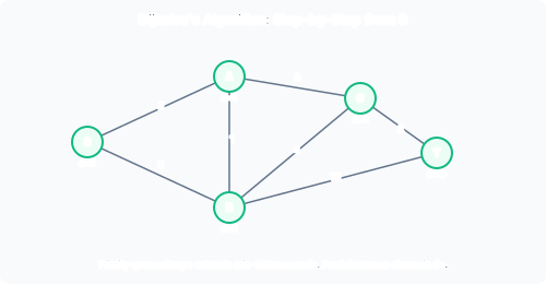
      Dijkstra algorithm worked example with final shortest-path distances

      Worked Example

      Same graph used in the Bellman-Ford notes: V={A,B,C,D,E,F,G}V = \{A,B,C,D,E,F,G\}, source s=Es = E, all weights non-negative.

      Edges: EA:5E \to A:5, EF:7E \to F:7, EG:3E \to G:3, AB:1A \to B:1, AC:2A \to C:2, GF:3G \to F:3, CD:2C \to D:2.

      IterExtractSd[A]d[A]d[B]d[B]d[C]d[C]d[D]d[D]d[E]d[E]d[F]d[F]d[G]d[G]
      Init\emptyset\infty\infty\infty\infty0\infty\infty
      1E{E}5\infty\infty\infty073
      2G{E,G}5\infty\infty\infty063
      3A{E,G,A}567\infty063
      4B{E,G,A,B}567\infty063
      5F{E,G,A,B,F}567\infty063
      6C{E,G,A,B,F,C}5679063
      7Dall5679063

      Extract order (by minimum dd): E(0), G(3), A(5), B(6), F(6), C(7), D(9). Note that B and F both have d=6d=6; tie-breaking is arbitrary. At each step, the extracted vertex’s distance is final: no later relaxation can reduce it.

      Shortest path from EE to DD: EACDE \to A \to C \to D (cost 5+2+2=95+2+2 = 9).

      Comparison with Bellman-Ford on the Same Graph

      Bellman-Ford takes up to 7 iterations of relaxing all edges. On this graph it converges in 2 iterations (since the longest shortest path has 3 edges, but convergence can be faster depending on edge order). Dijkstra extracts exactly V=7|V| = 7 vertices, each with one priority queue extract-min and neighbour relaxation. The extra overhead of the priority queue is offset by not scanning all edges on every iteration.

      Running Time Analysis

      Depends on the priority queue implementation:

      PQ ImplementationEXTRACT-MINDECREASE-KEYTotal
      Unsorted arrayO(V)O(V)O(1)O(1)O(V2+E)O(V^2 + E)
      Binary heapO(logV)O(\log V)O(logV)O(\log V)O((V+E)logV)O((V+E)\log V)
      Fibonacci heapO(logV)O(\log V) amortisedO(1)O(1) amortisedO(VlogV+E)O(V\log V + E)

      Derivation for binary heap: V|V| EXTRACT-MIN at O(logV)O(\log V) each; up to E|E| DECREASE-KEY at O(logV)O(\log V) each. Total: O(VlogV+ElogV)=O((V+E)logV)O(|V|\log|V| + |E|\log|V|) = O((|V|+|E|)\log|V|).

      For dense graphs where E=Θ(V2)|E| = \Theta(|V|^2), the array-based version (O(V2)O(|V|^2)) may outperform the binary heap version (O(V2logV)O(|V|^2 \log |V|)) due to lower constant factors. For sparse graphs, the heap methods are superior.

      Comparison with Bellman-Ford

      DijkstraBellman-Ford
      Edge weightsw0w \ge 0 onlyAny real
      TechniqueGreedy + PQDP / repeated relaxation
      TimeO((V+E)logV)O((V+E)\log V)O(VE)O(VE)
      Negative cycle detectionN/AYes
      Works on DAGsYesYes

      When Dijkstra Fails on Negative Edges

      Consider sas \to a (weight 2), sbs \to b (weight 3), aba \to b (weight 2-2). Dijkstra from ss: extracts aa first (d[a]=2d[a]=2), marking it final. Then relaxes (a,b)(a,b): d[b]=2+(2)=0d[b] = 2 + (-2) = 0. But bb‘s distance is now 0, whereas aa was finalised at 2 — the true shortest distance to aa might actually be via bb if we could go backwards (in a graph with more edges). The algorithm cannot backtrack to correct aa, so it produces wrong results. Bellman-Ford correctly handles this case.

      Summary

      PropertyDetail
      TypeGreedy algorithm
      Weight constraintw(u,v)0w(u,v) \ge 0 for all edges
      Data structurePriority queue (min-heap)
      Invariantv.d=δ(s,v)v.d = \delta(s,v) for all vSv \in S
      Binary heap timeO((V+E)logV)O((V+E)\log V)
      Fibonacci heap timeO(VlogV+E)O(V\log V + E)
      Fails onNegative edge weights

      Past paper questions: y2024p1q9 (opportunities, Dijkstra variants), y2023p1q9 (bidirectional Dijkstra), y2025p1q10(d) (Dijkstra with different priority queues).

    • Dijkstra's Algorithm: Correctness Proof

      The Induction Strategy

      We prove Dijkstra’s algorithm terminates with v.d=δ(s,v)v.d = \delta(s, v) for all vertices vv. The proof uses induction on the size of set SS (vertices whose distances have been finalised by extraction from the priority queue).

      Loop invariant Φ\Phi: At the start of each while-loop iteration, for every vertex vSv \in S, we have v.d=δ(s,v)v.d = \delta(s, v). That is, all vertices extracted so far have their correct shortest-path distances.

      Initialisation

      Before the first iteration, S=S = \emptyset, so Φ\Phi holds vacuously. The distance estimates are initialised: s.d=0=δ(s,s)s.d = 0 = \delta(s,s), and all other v.d=δ(s,v)v.d = \infty \ge \delta(s,v). The upper-bound property (analogous to BFS Lemma 2) holds: v.dv.d never underestimates the true distance.

      The Convergence Property of RELAX

      A supporting lemma used inside the proof:

      Convergence Property: If suvs \leadsto u \to v is a shortest path from ss to vv, and u.d=δ(s,u)u.d = \delta(s, u) before the edge (u,v)(u, v) is relaxed, then v.d=δ(s,v)v.d = \delta(s, v) after the relaxation.

      Proof: After relaxing (u,v)(u, v): v.du.d+w(u,v)=δ(s,u)+w(u,v)=δ(s,v)v.d \le u.d + w(u, v) = \delta(s, u) + w(u, v) = \delta(s, v) But we also have the upper-bound property v.dδ(s,v)v.d \ge \delta(s, v) at all times. Therefore v.d=δ(s,v)v.d = \delta(s, v) exactly.

      In words: if we already know the correct distance to uu, and (u,v)(u, v) is the last edge on a true shortest path to vv, then relaxing that edge pins down vv‘s correct distance.

      Maintenance: Proof by Contradiction

      Assume the invariant fails at some point. Let uu be the first vertex for which u.dδ(s,u)u.d \neq \delta(s, u) when it is added to SS.

      • usu \neq s, since s.d=0=δ(s,s)s.d = 0 = \delta(s, s) (correct).
      • There is a shortest path from ss to uu, because if uu were unreachable, u.d==δ(s,u)u.d = \infty = \delta(s, u), which would be correct.
      • SS \neq \emptyset at the moment uu is selected (it contains at least ss).

      Consider any shortest path p=sup = s \leadsto u. Let yy be the first vertex along pp (starting from ss) that is not yet in SS at the moment uu is selected. Let xSx \in S be yy‘s immediate predecessor on pp. Decompose:

      p=sp1xyp2up = s \underset{p_1}{\leadsto} x \to y \underset{p_2}{\leadsto} u

      Since xx was added to SS before uu, and uu is the first vertex where the invariant fails, we know x.d=δ(s,x)x.d = \delta(s, x). When xx was added to SS, the edge (x,y)(x, y) was relaxed. By the convergence property:

      y.d=δ(s,y)y.d = \delta(s, y)

      Now, because all edge weights are non-negative, and yy appears before uu on a shortest path: δ(s,y)δ(s,u)\delta(s, y) \le \delta(s, u)

      Because uu was the vertex with minimum dd value selected from the priority queue, and ySy \notin S as well: u.dy.du.d \le y.d

      Chaining these inequalities: δ(s,u)δ(s,y)=y.du.d\delta(s, u) \ge \delta(s, y) = y.d \ge u.d

      But the upper-bound property gives u.dδ(s,u)u.d \ge \delta(s, u). Together: u.d=δ(s,u)u.d = \delta(s, u)

      This contradicts the assumption that u.du.d was incorrect. Therefore the invariant Φ\Phi is maintained.

      Why Non-Negative Weights Are Essential

      The inequality δ(s,y)δ(s,u)\delta(s, y) \le \delta(s, u) relies on the fact that all edges on p2p_2 (from yy to uu) have non-negative weight. If any edge on p2p_2 were negative, the path yuy \leadsto u could have negative total weight, making δ(s,y)δ(s,u)\delta(s, y) \le \delta(s, u) false (it’s possible that uu is reachable from yy with a negative total, making δ(s,y)>δ(s,u)\delta(s, y) > \delta(s, u)). This is why Dijkstra fails on graphs with negative edges: the greedy choice of minimum dd is no longer guaranteed to be optimal.

      Termination

      When the while loop exits, the priority queue QQ is empty. Since Q=VSQ = V \setminus S, all vertices are now in SS. The invariant Φ\Phi holds for all vVv \in V, so v.d=δ(s,v)v.d = \delta(s, v) for every vertex. The algorithm is correct.

      The Predecessor Subgraph Is a Tree

      Because RELAX sets π[v]=u\pi[v] = u whenever a shorter path through uu is found, and the final dd values equal the true distances, the predecessor subgraph GπG_\pi (edges (π[v],v)(\pi[v], v) for vsv \neq s) is a shortest-path tree rooted at ss: a directed tree where the unique path from ss to any vertex is a shortest path in GG.

      Summary of Proof Structure

      StepMethod
      Invariantv.d=δ(s,v)v.d = \delta(s,v) for all vSv \in S
      BaseS=S = \emptyset, true vacuously
      Assumption for failureLet uu be first vertex added to SS with u.dδ(s,u)u.d \neq \delta(s,u)
      Construct counter-pathsxyus \leadsto x \to y \leadsto u where xSx \in S, ySy \notin S
      Key facts usedConvergence property; non-negative weights; u.dy.du.d \le y.d
      Contradictionδ(s,u)δ(s,y)=y.du.d\delta(s,u) \ge \delta(s,y) = y.d \ge u.d, so u.d=δ(s,u)u.d = \delta(s,u)
      ConclusionNo first failure → invariant holds for all

      Past paper questions: y2023p1q9 (bidirectional variant correctness), y2024p1q9 (relaxed costs and optimality).

    • Bellman-Ford Algorithm

      Overview

      Bellman-Ford solves the SSSP problem for graphs that may contain negative edge weights. The only restriction is that there be no negative-weight cycle reachable from the source (if one exists, shortest paths are undefined). The algorithm also explicitly detects negative cycles and reports failure.

      Unlike Dijkstra, which selects vertices greedily, Bellman-Ford relaxes every edge V1|V|-1 times. This brute-force approach ensures distances propagate correctly along all possible simple paths.

      Pseudocode

      BELLMAN-FORD(G, w, s):
        for each v in G.V:
          v.d = ∞
          v.π = NIL
        s.d = 0
        for i = 1 to |G.V| - 1:
          for each edge (u, v) in G.E:          // in any order
            RELAX(u, v, w)
        // Negative cycle detection pass
        for each edge (u, v) in G.E:
          if v.d > u.d + w(u, v):
            return FALSE                         // negative cycle exists
        return TRUE

      Why V1|V|-1 Iterations Suffice

      A simple shortest path has at most V1|V|-1 edges (no vertex is repeated). Consider a shortest path s=v0v1vk=ts = v_0 \to v_1 \to \cdots \to v_k = t with kV1k \le |V|-1.

      • After iteration 1: edge (v0,v1)(v_0, v_1) is relaxed, so d[v1]δ(s,v1)d[v_1] \le \delta(s, v_1). (In fact d[v1]=δ(s,v1)d[v_1] = \delta(s, v_1) if no shorter alternative exists.)
      • After iteration 2: edge (v1,v2)(v_1, v_2) is relaxed, so d[v2]δ(s,v2)d[v_2] \le \delta(s, v_2).
      • After iteration kk: d[t]δ(s,t)d[t] \le \delta(s, t).

      Since kV1k \le |V|-1, after V1|V|-1 iterations all vertices have d[v]=δ(s,v)d[v] = \delta(s, v). This can be formalised as dynamic programming: let d(k)[v]d^{(k)}[v] be the shortest path weight using at most kk edges. The recurrence d(k)[v]=min(d(k1)[v],min(u,v)E{d(k1)[u]+w(u,v)})d^{(k)}[v] = \min(d^{(k-1)}[v], \min_{(u,v) \in E} \{d^{(k-1)}[u] + w(u,v)\}) is exactly what the relaxation loop computes bottom-up.

      Negative Cycle Detection

      After V1|V|-1 passes over all edges, every d[v]d[v] should equal δ(s,v)\delta(s, v) (or \infty for unreachable vertices). If any edge can still be relaxed (i.e. v.d>u.d+w(u,v)v.d > u.d + w(u,v) for some (u,v)(u,v)), then:

      • There exists a path of length V\ge |V| whose weight decreases from the current dd values.
      • Such a path must contain at least V|V| edges, so it contains a cycle (by the pigeonhole principle).
      • Removing that cycle cannot increase path weight (or the path wouldn’t be shorter), so the cycle must have negative total weight.

      Thus a relaxable edge after V1|V|-1 passes indicates a negative-weight cycle reachable from ss.

      Important caveat: A negative cycle that is not reachable from ss will not be detected, because vertices in that component maintain d=d = \infty throughout and no edge from a finite-distance vertex enters the component. This does not affect the SSSP result for reachable vertices.

      Worked Example (No Negative Cycle)

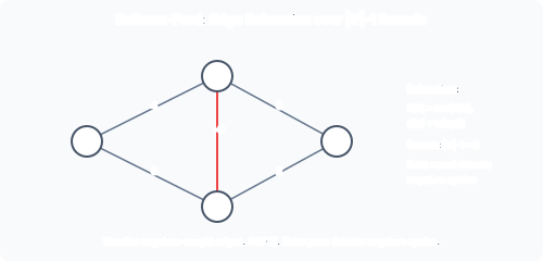
      Bellman-Ford algorithm: edge relaxation over multiple passes with a negative-weight edge

      Same graph as Dijkstra notes: V={A,B,C,D,E,F,G}V = \{A,B,C,D,E,F,G\}, source EE. Weights: EA:5E \to A:5, EF:7E \to F:7, EG:3E \to G:3, AB:1A \to B:1, AC:2A \to C:2, GF:3G \to F:3, CD:2C \to D:2.

      Processing edges in the order: (E,A), (E,F), (E,G), (A,B), (A,C), (G,F), (C,D).

      VertexIniti=1i=1i=2i=2i=36i=3\ldots6
      E0000
      A\infty5 (E)55
      B\infty\infty6 (A)6
      C\infty\infty7 (A)7
      D\infty\infty\infty9 (C)
      F\infty7 (E)6 (G)6
      G\infty3 (E)33

      After i=2i=2, all distances are final. Iterations 3-6 make no changes. Final check: no edge can be relaxed \to return TRUE.

      Worked Example (Negative Cycle)

      Modify the graph: change GFG \to F from 3 to 4-4, add edge DAD \to A with weight 7-7, add edge DCD \to C with weight 2-2. The cycle ACDAA \to C \to D \to A has weight 2+(2)+(7)=72 + (-2) + (-7) = -7 (negative).

      Run Bellman-Ford. After i=1i=1, d[C]d[C] is set to 7 (via A). After i=2i=2, d[D]d[D] is set to 5 (via C), and d[A]d[A] is set to 2-2 (via D). After i=3i=3, d[C]d[C] drops further, and so on. The values keep decreasing each iteration because the negative cycle propagates smaller distances indefinitely. After the full V1|V|-1 passes, the final check finds that some edge (e.g. (D,A)(D, A)) can still be relaxed. The algorithm returns FALSE.

      Early Termination and Practical Optimisations

      • If a complete pass over all edges produces no changes, all distances are final. The algorithm can terminate early. This does not improve the worst case but helps on well-behaved inputs.
      • Process edges in an order that respects topological order if the graph is a DAG (then only one pass is needed: DAG-SSSP in Θ(V+E)\Theta(V+E)).
      • Use a queue of vertices whose dd value changed in the previous pass (Shortest Path Faster Algorithm, SPFA), which often runs faster in practice though its worst case remains O(VE)O(VE).

      Running Time

      • Initialisation: Θ(V)\Theta(|V|).
      • Main loop: V1|V|-1 iterations, each scanning all E|E| edges: Θ(VE)\Theta(|V| \cdot |E|).
      • Final detection pass: Θ(E)\Theta(|E|).
      • Total: Θ(VE)\Theta(|V| \cdot |E|).

      For dense graphs: Θ(V3)\Theta(|V|^3). For sparse graphs: Θ(V2)\Theta(|V|^2) if E=Θ(V)|E| = \Theta(|V|).

      Comparison

      PropertyDijkstraBellman-Ford
      Edge weightsNon-negative onlyAny real
      Negative cycle detectionNoYes
      Time complexityO((V+E)logV)O((V+E)\log V)Θ(VE)\Theta(VE)
      Algorithm typeGreedyDynamic programming (implicit)
      Practical useFaster for w0w \ge 0Necessary for negative edges

      Summary

      PropertyDetail
      Weight constraintAny real numbers
      Negative cyclesDetected on final extra pass
      Why V1V-1 passesSimple shortest path has V1\le V-1 edges
      TimeΘ(VE)\Theta(V \cdot E)
      SpaceΘ(V)\Theta(V) beyond graph storage
      Convergence checkNo changes in a pass     \implies done

      Past paper questions: y2026p1q9(c,d) (undetected negative cycles, purpose of extra relaxation pass, early termination optimisation).

    • Johnson's Algorithm

      Overview

      Johnson’s algorithm solves the all-pairs shortest paths (APSP) problem for sparse graphs with possibly negative edge weights. It runs Bellman-Ford once to compute a potential function hh, uses hh to reweight all edges to non-negative values, then runs Dijkstra V|V| times. The original distances are recovered by subtracting the potential difference.

      The key insight: adding a constant to every edge weight does not preserve shortest paths (longer paths accumulate more bias). Instead, the bias must depend on the endpoints: w^(u,v)=w(u,v)+h(u)h(v)\hat{w}(u, v) = w(u, v) + h(u) - h(v).

      Why Naive Reweighting Fails

      Adding a fixed constant bb to every edge weight makes all edges non-negative, but changes which paths are shortest. If two paths from AA to BB have 2 edges and 5 edges respectively, the 5-edge path accumulates 5b5b vs 2b2b, so the ranking can change. Johnson’s vertex-potential reweighting avoids this.

      The Reweighting Function

      Given a function h:VRh: V \to \mathbb{R}, define the reweighted edge weight:

      w^(u,v)=w(u,v)+h(u)h(v)\hat{w}(u, v) = w(u, v) + h(u) - h(v)

      Property 1 (shortest-path preservation): For any path p=v1v2vkp = v_1 \to v_2 \to \cdots \to v_k:

      w^(p)=i=1k1(w(vi,vi+1)+h(vi)h(vi+1))=w(p)+h(v1)h(vk)\hat{w}(p) = \sum_{i=1}^{k-1} (w(v_i, v_{i+1}) + h(v_i) - h(v_{i+1})) = w(p) + h(v_1) - h(v_k)

      The terms telescope: h(vi)h(v_i) and h(vi+1)-h(v_{i+1}) cancel for interior vertices. The difference h(v1)h(vk)h(v_1) - h(v_k) depends only on the endpoints, not the path. Therefore w^\hat{w} preserves the relative ordering of paths between any fixed pair of vertices: a shortest path under ww is also a shortest path under w^\hat{w}.

      Property 2 (non-negative weights): If h(v)=δ(s,v)h(v) = \delta(s, v) (the true shortest distance from some source ss), then by the triangle inequality δ(s,v)δ(s,u)+w(u,v)\delta(s, v) \le \delta(s, u) + w(u, v), so:

      w^(u,v)=w(u,v)+h(u)h(v)0\hat{w}(u, v) = w(u, v) + h(u) - h(v) \ge 0

      Algorithm

      1. Augment GG to GG': add a new vertex ss connected to every vVv \in V with weight 0. GG' has no new negative cycles.
      2. Run Bellman-Ford on GG' from ss. If it detects a negative cycle, report failure. Otherwise, set h(v)=δ(s,v)h(v) = \delta(s, v) for all vv.
      3. Reweight every original edge: w^(u,v)=w(u,v)+h(u)h(v)\hat{w}(u, v) = w(u, v) + h(u) - h(v). Now all edges have non-negative weight.
      4. For each vertex uVu \in V, run Dijkstra on the reweighted graph to get δ^(u,v)\hat{\delta}(u, v) for all vv.
      5. Recover true distances: δ(u,v)=δ^(u,v)h(u)+h(v)\delta(u, v) = \hat{\delta}(u, v) - h(u) + h(v).

      Pseudocode:

      JOHNSON(G, w):
        G' = (V ∪ {s}, E ∪ {(s,v) : v ∈ V}) with w(s,v)=0
        if BELLMAN-FORD(G', w, s) == FALSE:
          error("negative cycle")
        for each edge (u,v) in G.E:
          ŵ(u,v) = w(u,v) + u.d - v.d      // u.d = δ(s,u)
        D = new |V|×|V| matrix
        for each u in G.V:
          DIJKSTRA(G, ŵ, u)
          for each v in G.V:
            D[u][v] = v.d - u.h + v.h        // undo reweighting
        return D

      Worked Example

      Consider a graph with V={1,2,3}V = \{1,2,3\} and edges: 121 \to 2 (weight 2-2), 131 \to 3 (weight 44), 232 \to 3 (weight 11). This has a negative edge 121 \to 2 but no negative cycles.

      Step 1: Augment with ss, edges s1,s2,s3s \to 1, s \to 2, s \to 3 (weight 0).

      Step 2: Bellman-Ford from ss gives h(1)=0h(1)=0, h(2)=0h(2)=0, h(3)=0h(3)=0 (there are no paths to improve, since ss edges are 0-weight). Actually, with the original edges present: h(1)=0h(1)=0, h(2)=2h(2)=-2, h(3)=1h(3)=-1 (path s123s \to 1 \to 2 \to 3 costs 02+1=10-2+1=-1, or s13s \to 1 \to 3 costs 44).

      Step 3: Reweight:

      • w^(1,2)=2+0(2)=0\hat{w}(1,2) = -2 + 0 - (-2) = 0
      • w^(1,3)=4+0(1)=5\hat{w}(1,3) = 4 + 0 - (-1) = 5
      • w^(2,3)=1+(2)(1)=0\hat{w}(2,3) = 1 + (-2) - (-1) = 0

      All reweighted edges are non-negative.

      Step 4: Run Dijkstra from 1: δ^(1,2)=0\hat{\delta}(1,2)=0, δ^(1,3)=0\hat{\delta}(1,3)=0 (via 1231 \to 2 \to 3).

      Step 5: Recover: δ(1,2)=00+(2)=2\delta(1,2) = 0 - 0 + (-2) = -2, δ(1,3)=00+(1)=1\delta(1,3) = 0 - 0 + (-1) = -1.

      Results match the original graph (path 1231 \to 2 \to 3 costs 2+1=1-2+1=-1).

      Running Time

      • Step 1: Θ(V)\Theta(|V|).
      • Step 2: Θ(VE)\Theta(|V|\cdot|E|) (Bellman-Ford).
      • Step 3: Θ(E)\Theta(|E|).
      • Step 4: V|V| calls to Dijkstra. With binary heap: O(V(V+E)logV)=O(VElogV)O(|V| \cdot (|V|+|E|)\log|V|) = O(|V| \cdot |E| \log |V|). With Fibonacci heap: O(V2logV+VE)O(|V|^2 \log |V| + |V| \cdot |E|).
      • Step 5: Θ(V2)\Theta(|V|^2).

      Total: O(V2logV+VE)O(|V|^2 \log |V| + |V| \cdot |E|) with Fibonacci heap, or O(VElogV)O(|V| \cdot |E| \log |V|) with binary heap.

      Comparison with Floyd-Warshall

      AlgorithmTimeBest for
      JohnsonO(V2logV+VE)O(V^2 \log V + VE)Sparse graphs
      Floyd-WarshallΘ(V3)\Theta(V^3)Dense graphs

      Johnson wins when E=o(V2)|E| = o(|V|^2). When E=Θ(V2)|E| = \Theta(|V|^2), Floyd-Warshall’s simpler implementation and smaller constant factor make it preferable.

      Summary

      StepOperationTime
      AugmentAdd dummy ssO(V)O(V)
      Bellman-FordCompute h(v)h(v)O(VE)O(VE)
      Reweightw^=w+h(u)h(v)\hat{w} = w + h(u) - h(v)O(E)O(E)
      Dijkstra × VVAll-pairsO(VElogV)O(V \cdot E \log V)
      Un-reweightD[u][v]+h(u)h(v)D[u][v] + h(u) - h(v)O(V2)O(V^2)

      Past paper questions: y2024p1q9 (reweighting, relaxed costs, opportunities).

    • Floyd-Warshall Algorithm

      Overview

      Floyd-Warshall solves the all-pairs shortest paths (APSP) problem using dynamic programming. It is particularly suited to dense graphs, running in Θ(V3)\Theta(|V|^3) time and Θ(V2)\Theta(|V|^2) space (in-place optimisation). It handles negative edge weights but, like all shortest-path algorithms, requires that no negative-weight cycles exist.

      The DP Recurrence

      Number the vertices 1,2,,n1, 2, \ldots, n. Let dij(k)d_{ij}^{(k)} be the weight of a shortest path from ii to jj using only intermediate vertices from the set {1,2,,k}\{1, 2, \ldots, k\}. The base case k=0k=0 uses no intermediate vertices:

      dij(0)={0if i=jw(i,j)if (i,j)Eotherwised_{ij}^{(0)} = \begin{cases} 0 & \text{if } i = j \\ w(i, j) & \text{if } (i, j) \in E \\ \infty & \text{otherwise} \end{cases}

      For k1k \ge 1, vertex kk is either used as an intermediate vertex or not:

      dij(k)=min(dij(k1),  dik(k1)+dkj(k1))d_{ij}^{(k)} = \min\left(d_{ij}^{(k-1)},\; d_{ik}^{(k-1)} + d_{kj}^{(k-1)}\right)

      After k=nk = n, we have the full all-pairs shortest distances.

      Pseudocode

      FLOYD-WARSHALL(W):
        n = number of vertices
        D^(0) = W            // W is the weight matrix (∞ for absent edges)
        for k = 1 to n:
          let D^(k) be a new n × n matrix
          for i = 1 to n:
            for j = 1 to n:
              D^(k)[i][j] = min(D^(k-1)[i][j],
                                D^(k-1)[i][k] + D^(k-1)[k][j])
        return D^(n)

      Space optimisation: The D(k1)D^{(k-1)} matrix can be overwritten to produce D(k)D^{(k)} in place because dik(k1)=dik(k)d_{ik}^{(k-1)} = d_{ik}^{(k)} and dkj(k1)=dkj(k)d_{kj}^{(k-1)} = d_{kj}^{(k)} (paths where kk is an intermediate vertex cannot have kk as an endpoint). So a single n×nn \times n matrix suffices.

      Worked Example

      Consider a graph with V={1,2,3,4}V = \{1,2,3,4\}, edges and weights:

      W=D(0)=(03780250120)W = D^{(0)} = \begin{pmatrix} 0 & 3 & \infty & 7 \\ 8 & 0 & 2 & \infty \\ 5 & \infty & 0 & 1 \\ 2 & \infty & \infty & 0 \end{pmatrix}

      k=1k=1 (intermediate vertex {1}):

      • d2,3(1)=min(d2,3(0),d2,1(0)+d1,3(0))=min(2,8+)=2d_{2,3}^{(1)} = \min(d_{2,3}^{(0)}, d_{2,1}^{(0)} + d_{1,3}^{(0)}) = \min(2, 8+\infty) = 2
      • d2,4(1)=min(,8+7)=15d_{2,4}^{(1)} = \min(\infty, 8+7) = 15
      • d3,2(1)=min(,5+3)=8d_{3,2}^{(1)} = \min(\infty, 5+3) = 8
      • d4,2(1)=min(,2+3)=5d_{4,2}^{(1)} = \min(\infty, 2+3) = 5

      D(1)=(037802155801250)D^{(1)} = \begin{pmatrix} 0 & 3 & \infty & 7 \\ 8 & 0 & 2 & 15 \\ 5 & 8 & 0 & 1 \\ 2 & 5 & \infty & 0 \end{pmatrix}

      k=2k=2 (intermediate vertices {1,2}):

      • d1,3(2)=min(,3+2)=5d_{1,3}^{(2)} = \min(\infty, 3+2) = 5
      • d3,4(2)=min(1,8+15)=1d_{3,4}^{(2)} = \min(1, 8+15) = 1
      • d4,3(2)=min(,5+2)=7d_{4,3}^{(2)} = \min(\infty, 5+2) = 7

      D(2)=(03578021558012570)D^{(2)} = \begin{pmatrix} 0 & 3 & 5 & 7 \\ 8 & 0 & 2 & 15 \\ 5 & 8 & 0 & 1 \\ 2 & 5 & 7 & 0 \end{pmatrix}

      k=3k=3 (intermediate vertices {1,2,3}):

      • d4,4(3)=min(0,7+1)=min(0,8)=0d_{4,4}^{(3)} = \min(0, 7+1) = \min(0,8) = 0 (no change).

      D(3)=(same as D(2), no new paths)D^{(3)} = \text{(same as $D^{(2)}$, no new paths)}

      k=4k=4:

      • d1,4(4)=min(7,7+0)=7d_{1,4}^{(4)} = \min(7, 7+0) = 7 (unchanged)
      • All others checked; no improvements.

      D(4)=D(2)D^{(4)} = D^{(2)}

      The final matrix gives all-pairs distances. For example, δ(4,3)=7\delta(4,3) = 7 via path 41234 \to 1 \to 2 \to 3 (cost 2+3+2=72+3+2=7).

      Predecessor Matrix

      To reconstruct paths, maintain a predecessor matrix Π(k)\Pi^{(k)} in parallel. Initialise πij(0)=i\pi_{ij}^{(0)} = i if (i,j)E(i,j) \in E or i=ji = j, else NIL. Update alongside the distance matrix: if the dik+dkjd_{ik} + d_{kj} path is chosen, set πij(k)=πkj(k1)\pi_{ij}^{(k)} = \pi_{kj}^{(k-1)}.

      Transitive Closure

      Floyd-Warshall can compute the transitive closure GG^* of a graph: an edge (i,j)(i,j) exists in GG^* iff there is a path from ii to jj in GG. Replace MIN with logical OR and ++ with logical AND. Initialise dij(0)=1d_{ij}^{(0)} = 1 if i=ji = j or (i,j)E(i,j) \in E, 0 otherwise. Running the same triple loop yields the reachability matrix in Θ(V3)\Theta(|V|^3).

      For DAGs, the transitive closure can be computed more efficiently by processing vertices in topological order.

      Comparison with Johnson

      AlgorithmTimeSpaceBest for
      Floyd-WarshallΘ(V3)\Theta(V^3)Θ(V2)\Theta(V^2)Dense graphs
      JohnsonO(V2logV+VE)O(V^2 \log V + VE)Θ(V2)\Theta(V^2)Sparse graphs

      When E=Θ(V2)|E| = \Theta(|V|^2), both are Θ(V3)\Theta(|V|^3), but Floyd-Warshall has lower constant factors and is simpler to implement.

      Summary

      PropertyDetail
      TypeDynamic programming
      Recurrencedij(k)=min(dij(k1),dik(k1)+dkj(k1))d_{ij}^{(k)} = \min(d_{ij}^{(k-1)}, d_{ik}^{(k-1)} + d_{kj}^{(k-1)})
      Base casedij(0)=w(i,j)d_{ij}^{(0)} = w(i,j) or 0 for i=ji=j
      TimeΘ(V3)\Theta(V^3)
      SpaceΘ(V2)\Theta(V^2) (in-place)
      Negative weightsHandled (no negative cycles)
      Transitive closureReplace min/+ with OR/AND

      Past paper questions: y2026p1q10(c,d) (DAG transitive closure optimisation).

  • Strongly Connected Components

    Kosaraju's algorithm for finding strongly connected components in directed graphs

    • Strongly Connected Components

      Definition

      A strongly connected component (SCC) of a directed graph G=(V,E)G = (V, E) is a maximal subset CVC \subseteq V such that for every ordered pair of vertices u,vCu, v \in C, there exists a directed path from uu to vv and a directed path from vv to uu. In other words, every vertex in the SCC can reach every other vertex within the SCC.

      SCCs form a partition of the vertex set: every vertex belongs to exactly one SCC. A singleton vertex with no self-loop is a trivial SCC of size 1. SCCs generalise the notion of connected components from undirected graphs to directed graphs, requiring bidirectional reachability rather than just undirected connectivity.

      Worked Example

      Directed graph: V={1,2,3,4,5,6,7,8}V = \{1,2,3,4,5,6,7,8\}, edges:

      121 \to 2, 232 \to 3, 242 \to 4, 313 \to 1, 343 \to 4, 434 \to 3, 545 \to 4, 565 \to 6, 656 \to 5, 676 \to 7, 787 \to 8, 868 \to 6, 878 \to 7.

      SCC decomposition:

      • SCC 1: {1,2,3,4}\{1, 2, 3, 4\}. Vertices 1, 2, 3, 4 are all mutually reachable: 12311 \to 2 \to 3 \to 1 forms a directed cycle; 3433 \to 4 \to 3 is another cycle; 242 \to 4 is within the same SCC since 43124 \to 3 \to 1 \to 2 gives the return path. Edges to vertices outside: 545 \to 4 enters this SCC.
      • SCC 2: {5,6,7,8}\{5, 6, 7, 8\}. 5655 \to 6 \to 5 is a cycle; 67866 \to 7 \to 8 \to 6 is another cycle. All four are mutually reachable.

      Thus the graph has two SCCs.

      The Component Graph

      Define the component graph GSCC=(VSCC,ESCC)G^{\text{SCC}} = (V^{\text{SCC}}, E^{\text{SCC}}):

      • Each vertex in VSCCV^{\text{SCC}} corresponds to one SCC of GG.
      • A directed edge CiCjC_i \to C_j exists iff there is at least one edge (u,v)E(u, v) \in E where uCiu \in C_i and vCjv \in C_j (i.e. there is an edge from some vertex in CiC_i to some vertex in CjC_j in the original graph).

      Theorem: GSCCG^{\text{SCC}} is always a DAG (directed acyclic graph).

      Proof: Suppose GSCCG^{\text{SCC}} contained a directed cycle C1C2CkC1C_1 \to C_2 \to \cdots \to C_k \to C_1. Then:

      • A vertex in C1C_1 can reach a vertex in C2C_2 (by the original graph edges).
      • A vertex in C2C_2 can reach a vertex in C3C_3.
      • A vertex in CkC_k can reach a vertex in C1C_1.

      By transitivity of reachability, every vertex in C1C2CkC_1 \cup C_2 \cup \cdots \cup C_k can reach every other vertex in this union. But then i=1kCi\bigcup_{i=1}^k C_i would itself be strongly connected, contradicting the maximality of the SCCs (they would have been merged into a single larger SCC). Hence GSCCG^{\text{SCC}} is acyclic.

      Since the component graph is a DAG, it has at least one source SCC (no incoming edges from other SCCs) and at least one sink SCC (no outgoing edges to other SCCs). It also admits a topological ordering.

      Properties

      1. SCCs are closed under cycles: Any directed cycle is entirely contained within a single SCC.
      2. Condensation: Collapsing each SCC into a single super-node produces the component graph, which is a DAG. Many graph problems become simpler on the condensed graph.
      3. DFS and SCCs: DFS on a directed graph assigns finish times that respect the topological ordering of the component graph: vertices in a “downstream” SCC (closer to a sink) finish before vertices in an “upstream” SCC.

      Why SCCs Matter

      • Cycle analysis: If a graph has cycles, they are contained within SCCs. Reducing the graph to its component DAG reveals the acyclic structure.
      • Social networks: Mutual follow groups correspond to SCCs.
      • Deadlock detection: In a wait-for graph of processes/resources, cycles indicate deadlocks. The SCC decomposition identifies all deadlocked groups.
      • Graph compression: A large graph can be compressed by replacing each SCC with a single representative node.
      • Logic and compilation: Dependency graphs for modules or SAT solvers often contain SCCs; collapsing them simplifies analysis.

      Algorithms to Find SCCs

      AlgorithmTechniqueTime
      KosarajuTwo-pass DFS (GG then GTG^T)Θ(V+E)\Theta(V+E)
      TarjanSingle-pass DFS with lowlinksΘ(V+E)\Theta(V+E)

      Only Kosaraju is on the Part IA syllabus. See Kosaraju’s Algorithm for the full treatment.

      Relationship with Other Concepts

      • Weakly connected components (undirected sense) can span multiple SCCs. SCC is a stricter notion of connectivity.
      • DAGs: Every vertex in a DAG is its own SCC (there are no cycles, so no nontrivial mutual reachability). The component graph of a DAG is isomorphic to the DAG itself.
      • Topological sort: Works on DAGs. For a general directed graph, topologically sort the component graph, then topologically sort within each SCC (though within an SCC no total order respecting all edges can exist since there are cycles).

      Summary

      TermDefinition
      SCCMaximal mutually reachable vertex set
      Component graphDAG where each node = one SCC
      CondensationCollapsing SCCs yields DAG
      KosarajuTwo-pass DFS, Θ(V+E)\Theta(V+E)
      Key propertyGSCCG^{\text{SCC}} is always acyclic
      DFS propertyFinish times reflect component DAG topological order

      Past paper questions: SCCs are assessed conceptually; Kosaraju’s steps may appear in open-ended algorithm questions. Also see y2026p1q10 (DAG).

    • Kosaraju's Algorithm

      Overview

      Kosaraju's algorithm: two strongly connected components separated by a bridge edge

      Kosaraju’s algorithm finds all strongly connected components (SCCs) of a directed graph in Θ(V+E)\Theta(|V| + |E|) time using two complete passes of DFS. It is elegant and requires only basic DFS, making it a natural exam topic.

      Algorithm: Three Steps

      1. DFS on GG: Run a full DFS on the original graph GG. Record the finish time f[v]f[v] for every vertex.
      2. Transpose: Compute the transpose graph GTG^T: reverse the direction of every edge. VT=VV^T = V, ET={(v,u)(u,v)E}E^T = \{(v,u) \mid (u,v) \in E\}.
      3. DFS on GTG^T: Run DFS on GTG^T, but in the outer loop (which picks the next root), process vertices in decreasing order of their finish times from step 1. Each DFS tree in this forest is one SCC of GG.

      Pseudocode

      KOSARAJU(G):
        // Step 1: DFS on G, record finish times
        for each v in G.V:
          v.colour = WHITE
          v.π = NIL
        time = 0
        order = []                 // list for finish-time ordering
        for each v in G.V:
          if v.colour == WHITE:
            DFS-VISIT-FINISH(G, v, order)
      
        // Step 2: Compute G^T
        GT = TRANSPOSE(G)
      
        // Step 3: DFS on G^T in reverse finish order
        for each v in GT.V:
          v.colour = WHITE
        sccs = []
        for each v in reverse(order):  // decreasing finish time
          if v.colour == WHITE:
            component = []
            DFS-VISIT-COLLECT(GT, v, component)
            sccs.append(component)
        return sccs

      Intuition

      Why does processing GTG^T in decreasing finish-time order produce SCCs?

      • In step 1, DFS on GG assigns finish times. The SCC that acts as a sink in the component DAG (no outgoing edges to other SCCs) finishes first amongst its DFS tree. More generally, finish times reveal the topological order of the component DAG: components earlier in the topological order finish later.
      • In step 3, we reverse all edges. The sink SCC in GG becomes a source SCC in GTG^T. Since we process vertices in decreasing finish order, we start DFS from a vertex in the “last-finishing” component (a sink in GG, source in GTG^T). Because edges between SCCs are reversed, the DFS cannot escape this SCC into others that haven’t been visited yet.
      • Within an SCC, edges go both ways, so reversing preserves strong connectivity: if vertices uu and vv are mutually reachable in GG, they remain mutually reachable in GTG^T.

      Worked Example

      Graph with V={1,2,3,4,5,6,7,8}V = \{1,2,3,4,5,6,7,8\} and edges (as in the SCC notes):

      121 \to 2, 232 \to 3, 242 \to 4, 313 \to 1, 343 \to 4, 434 \to 3, 545 \to 4, 565 \to 6, 656 \to 5, 676 \to 7, 787 \to 8, 868 \to 6, 878 \to 7.

      Step 1: DFS on GG, start at 1 (assume adjacency list order as listed). Discovery/finish times:

      Vertex12345678
      dd1234121385
      ff1615107111496

      (Values depend on adjacency order; any valid DFS is fine.) Decreasing finish order: 1,2,6,5,3,7,4,81, 2, 6, 5, 3, 7, 4, 8.

      Step 2: GTG^T. All edges reversed: 212 \to 1, 323 \to 2, 424 \to 2, 131 \to 3, 434 \to 3, 343 \to 4, 454 \to 5, 656 \to 5, 565 \to 6, 767 \to 6, 878 \to 7, 686 \to 8, 787 \to 8.

      Step 3: DFS on GTG^T, order: 1, 2, 6, 5, 3, 7, 4, 8.

      • Start from 1 (first in order). DFS from 1 reaches {1,3,4,2}\{1,3,4,2\}. This is SCC {1,2,3,4}\{1,2,3,4\}.
      • Next unvisited in order: 6. DFS from 6 reaches {6,5,8,7}\{6,5,8,7\}. This is SCC {5,6,7,8}\{5,6,7,8\}.
      • Result: two SCCs as expected.

      Time Complexity

      • DFS on GG: Θ(V+E)\Theta(|V| + |E|).
      • Computing GTG^T: Θ(V+E)\Theta(|V| + |E|) (reverse every edge).
      • DFS on GTG^T: Θ(V+E)\Theta(|V| + |E|).
      • Total: Θ(V+E)\Theta(|V| + |E|) — linear in the size of the graph.

      The algorithm is optimal: any algorithm must at least examine every vertex and edge to find all SCCs.

      Correctness Sketch

      Let C1C_1 and C2C_2 be two distinct SCCs of GG with an edge from C1C_1 to C2C_2 in the component DAG. In step 1, all vertices in C1C_1 finish after all vertices in C2C_2, assuming C1C_1 is explored first. More formally, the finish-time ordering corresponds to a reverse topological sort of the component DAG. Thus, when we process GTG^T in decreasing finish order, we first explore a sink SCC of GG (now a source in GTG^T), and edges to other SCCs point the opposite way in GTG^T, so the DFS stays within the current SCC. The official proof is in CLRS Chapter 22.

      Summary

      StepActionTime
      1DFS on GG, record f[v]f[v]Θ(V+E)\Theta(V+E)
      2Construct GTG^TΘ(V+E)\Theta(V+E)
      3DFS on GTG^T, decreasing f[v]f[v] orderΘ(V+E)\Theta(V+E)
      TotalΘ(V+E)\Theta(V+E)

      Past paper questions: SCCs are assessed conceptually; Kosaraju’s algorithm may appear as a direct algorithm question or as part of a larger problem.

  • Maximum Flow

    Flow networks, the Ford-Fulkerson method, max-flow min-cut theorem, Edmonds-Karp, and reduction of bipartite matching to max flow

    • Flow Networks and the Maximum-Flow Problem

      A flow network models the movement of a commodity (oil, water, data) through a network with capacity constraints. The problem is to maximise throughput from source to sink.

      Definitions

      A flow network is a directed graph G=(V,E)G = (V, E) with two distinguished vertices:

      • Source sVs \in V: origin of flow, no incoming flow
      • Sink tVt \in V: destination of flow, no outgoing flow

      Each edge (u,v)E(u, v) \in E has a non-negative capacity c(u,v)0c(u, v) \ge 0. We assume no self-loops and (for convenience) no antiparallel edges: if (u,v)E(u, v) \in E then (v,u)E(v, u) \notin E. Antiparallel edges can be removed by inserting a dummy vertex. Every vertex lies on some path svts \leadsto v \leadsto t.

      Flow

      A flow f:V×VRf: V \times V \to \mathbb{R} satisfies:

      1. Capacity constraint: 0f(u,v)c(u,v)0 \le f(u, v) \le c(u, v) for all u,vVu, v \in V
      2. Flow conservation: for every vertex uV{s,t}u \in V \setminus \{s, t\}:

      vVf(v,u)=vVf(u,v)\sum_{v \in V} f(v, u) = \sum_{v \in V} f(u, v)

      Total flow in equals total flow out at every internal vertex. We define f(u,v)=0f(u, v) = 0 if (u,v)E(u, v) \notin E.

      The value of flow ff is the net flow leaving the source:

      f=vVf(s,v)vVf(v,s)|f| = \sum_{v \in V} f(s, v) - \sum_{v \in V} f(v, s)

      The second sum is usually zero but is included for generality.

      Antisymmetry Convention

      For notational convenience, define f(v,u)=f(u,v)f(v, u) = -f(u, v). This lets us write net flow across a cut as a single sum. In practice, flow only exists in forward directions up to capacity; the antisymmetry notion simplifies the algebra of residual networks.

      Residual Networks

      Given flow ff on GG, the residual network Gf=(V,Ef)G_f = (V, E_f) shows how much additional flow can be pushed on each edge, and where flow can be cancelled:

      • If (u,v)E(u, v) \in E and f(u,v)<c(u,v)f(u, v) < c(u, v), add (u,v)(u, v) to EfE_f with residual capacity cf(u,v)=c(u,v)f(u,v)c_f(u, v) = c(u, v) - f(u, v)
      • If f(u,v)>0f(u, v) > 0 (i.e. (v,u)E(v, u) \in E with positive flow), add (v,u)(v, u) to EfE_f with cf(v,u)=f(u,v)c_f(v, u) = f(u, v)

      Residual edges in the reverse direction represent flow cancellation: we can “undo” flow previously sent along the forward edge.

      Formally:

      cf(u,v)={c(u,v)f(u,v)if (u,v)Ef(v,u)if (v,u)E0otherwisec_f(u, v) = \begin{cases} c(u, v) - f(u, v) & \text{if } (u, v) \in E \\ f(v, u) & \text{if } (v, u) \in E \\ 0 & \text{otherwise} \end{cases}

      Augmentation

      If ff' is a flow in GfG_f, then the augmented flow fff \uparrow f' is:

      (ff)(u,v)=f(u,v)+f(u,v)f(v,u)(f \uparrow f')(u, v) = f(u, v) + f'(u, v) - f'(v, u)

      This yields a valid flow in GG with value ff=f+f|f \uparrow f'| = |f| + |f'|.

      Problem Statement

      Maximum-Flow Problem: given a flow network G=(V,E)G = (V, E) with capacities cc, source ss, and sink tt, find a flow ff of maximum value f|f|.

      Applications

      • Transport and logistics networks
      • Bipartite matching (see Maximum Bipartite Matching via Flow)
      • Circulation with demands
      • Image segmentation (min-cut formulation)
      • Edge-disjoint and vertex-disjoint paths
      • Project selection / maximum closure
      • Baseball elimination

      Antiparallel Edge Elimination

      If (u,v)(u, v) and (v,u)(v, u) both exist with capacities aa and bb, insert a new vertex xx and replace (v,u)(v, u) with (v,x)(v, x) and (x,u)(x, u), both of capacity bb. The resulting network has no antiparallel edges and preserves all feasible flows.

      Example

      Consider a simple 4-vertex network:

      • sas \to a (capacity 10), sbs \to b (capacity 5)
      • aba \to b (capacity 3), ata \to t (capacity 8)
      • btb \to t (capacity 7)

      Simple flow network

      A feasible flow sends 8 via sats \to a \to t and 7 via sbts \to b \to t, but the aba \to b edge capacity of 3 constrains redistribution. The maximum flow value is 15 (send 10 on sas \to a, split 8 to tt and 2 via bb, plus 5 from sbs \to b, total 8+2+5=158 + 2 + 5 = 15).

      Summary

      ConceptDefinition
      Flow networkG=(V,E)G = (V, E) with source ss, sink tt, capacities c(u,v)0c(u, v) \ge 0
      Capacity constraint0f(u,v)c(u,v)0 \le f(u, v) \le c(u, v)
      Flow conservationvf(v,u)=vf(u,v)\sum_v f(v, u) = \sum_v f(u, v) for us,tu \neq s, t
      Flow value f\lvert f \rvertNet flow out of ss: vf(s,v)vf(v,s)\sum_v f(s, v) - \sum_v f(v, s)
      Residual capacitycf(u,v)=c(u,v)f(u,v)+f(v,u)c_f(u, v) = c(u, v) - f(u, v) + f(v, u)
      Augmentationfff \uparrow f' adds residual flow ff' to ff

      Past Tripos: y2024p1q9, y2023p2q7.

    • The Ford-Fulkerson Method

      The Ford-Fulkerson method is the foundational approach to solving the maximum-flow problem. It repeatedly finds paths from source to sink in the residual network and augments flow along them.

      Core Idea

      Start with zero flow. While an augmenting path (a simple path from ss to tt in the residual network GfG_f) exists, compute the bottleneck capacity along that path and push that amount of additional flow through every edge of the path.

      Algorithm

      FORD-FULKERSON(G, s, t):
          initialise flow f = 0 on all edges
          while there exists an augmenting path p in G_f:
              c_f(p) = min{ c_f(u, v) | (u, v) on p }
              for each edge (u, v) on p:
                  if (u, v) in G.E:
                      f(u, v) = f(u, v) + c_f(p)
                  else:
                      f(v, u) = f(v, u) - c_f(p)
          return f

      When processing a residual edge that corresponds to a reverse direction, we decrease the forward flow (cancelling it), effectively “pushing flow backwards”.

      Finding Augmenting Paths

      Any graph search (DFS or BFS) on GfG_f suffices. DFS may produce long, meandering paths; BFS finds shortest augmenting paths (in number of edges) and leads to the Edmonds-Karp variant.

      Worked Example

      Consider this network (edge labels show capacity):

          s ---10--> a ---3--> b ---7--> t
          |         |                  ^
          +----5--->b-----------------+
                    a ---8--> t

      Initial flow is zero everywhere. Residual network equals original.

      Iteration 1: augmenting path sats \to a \to t, bottleneck min(10,8)=8\min(10, 8) = 8. Flow: f(s,a)=8f(s, a) = 8, f(a,t)=8f(a, t) = 8. Residual: (s,a)(s, a) has residual 2, (a,t)(a, t) has residual 0, plus reverse edges (a,s)(a, s) capacity 8, (t,a)(t, a) capacity 8.

      Iteration 2: augmenting path sbts \to b \to t, bottleneck min(5,7)=5\min(5, 7) = 5. Flow: f(s,b)=5f(s, b) = 5, f(b,t)=5f(b, t) = 5. Residual: (s,b)(s, b) has residual 0, (b,t)(b, t) has residual 2.

      Iteration 3: augmenting path sabts \to a \to b \to t, bottleneck min(2,3,2)=2\min(2, 3, 2) = 2. Flow: f(s,a)=10f(s, a) = 10, f(a,b)=2f(a, b) = 2, f(b,t)=7f(b, t) = 7. Residual: (s,a)(s, a) saturated, (b,t)(b, t) saturated, (a,b)(a, b) has residual 1.

      No further augmenting paths exist. Maximum flow value =8+5+2=15= 8 + 5 + 2 = 15.

      The residual network at termination shows ss can only reach {a}\{a\}; sink tt is unreachable. This partition is a minimum cut (see Max-Flow Min-Cut Theorem).

      Termination and Running Time

      Integer Capacities

      If all capacities are integers, each augmentation increases f|f| by at least 1. Since f|f| \le total capacity out of ss, at most f|f^*| augmentations, where ff^* is the maximum flow. Cost per augmentation: O(E)O(|E|) for DFS/BFS. Total: O(Ef)O(|E| \cdot |f^*|).

      This is pseudopolynomial: the running time depends on the numeric value of the capacities, not just the graph size. For a network where f|f^*| is large (e.g. capacity 10910^9), this is impractical.

      Irrational Capacities

      With irrational capacities, Ford-Fulkerson with arbitrary path selection may fail to terminate. The flow can increase by ever-smaller increments in a non-convergent series. This is a theoretical concern only; all practical implementations use rational capacities.

      Practical Considerations

      Always use BFS (Edmonds-Karp) or Dinic’s algorithm. Never use arbitrary DFS path selection in real code. See Edmonds-Karp Algorithm for the polynomial-time variant.

      Summary

      AspectDetail
      Core operationFind augmenting path in GfG_f, push bottleneck capacity
      Flow cancellationReverse edges in GfG_f allow “undoing” flow
      Termination (integer)O(Ef)O(\lvert E \rvert \cdot \lvert f^* \rvert) — pseudopolynomial
      Termination (irrational)Not guaranteed
      Key insightResidual network encodes all possible flow adjustments

      Past Tripos: y2024p1q9, y2022p2q7.

    • The Max-Flow Min-Cut Theorem

      The Max-Flow Min-Cut Theorem is the central result of flow networks. It states that the maximum value of a flow equals the minimum capacity of a cut separating ss from tt, and it provides a constructive verification: when Ford-Fulkerson terminates, the set of vertices reachable from ss in the residual network is a minimum cut.

      Cuts

      An (s,t)(s, t)-cut of a flow network is a partition of VV into sets SS and T=VST = V \setminus S such that sSs \in S and tTt \in T.

      The net flow across the cut is:

      f(S,T)=uSvTf(u,v)uSvTf(v,u)f(S, T) = \sum_{u \in S} \sum_{v \in T} f(u, v) - \sum_{u \in S} \sum_{v \in T} f(v, u)

      The capacity of the cut (ignoring flow direction from TT to SS) is:

      c(S,T)=uSvTc(u,v)c(S, T) = \sum_{u \in S} \sum_{v \in T} c(u, v)

      Fundamental Lemma

      For any flow ff and any cut (S,T)(S, T):

      f=f(S,T)c(S,T)|f| = f(S, T) \le c(S, T)

      Proof sketch: f=f(S,T)|f| = f(S, T) follows from flow conservation (all flow from ss to tt must cross the cut, and internal vertices contribute zero net flow). f(S,T)c(S,T)f(S, T) \le c(S, T) follows because each edge’s flow cannot exceed its capacity, and the second sum (from TT to SS) is non-negative.

      This immediately gives: max-flowmin-cut\max\text{-flow} \le \min\text{-cut}.

      The Theorem

      Max-Flow Min-Cut Theorem: The following are equivalent:

      1. ff is a maximum flow in GG
      2. The residual network GfG_f contains no augmenting paths
      3. f=c(S,T)|f| = c(S, T) for some cut (S,T)(S, T) of GG

      Proof of Equivalence

      (1)     \implies (2): If GfG_f had an augmenting path pp, augmenting along pp would yield a flow of value f+cf(p)>f|f| + c_f(p) > |f|, contradicting maximality.

      (2)     \implies (3): Since no path exists from ss to tt in GfG_f, define S={vVthere is a path from s to v in Gf}S = \{v \in V \mid \text{there is a path from } s \text{ to } v \text{ in } G_f\} and T=VST = V \setminus S. This is a cut (sSs \in S, tTt \in T). For any uS,vTu \in S, v \in T:

      • If (u,v)E(u, v) \in E, we must have f(u,v)=c(u,v)f(u, v) = c(u, v); otherwise (u,v)(u, v) would be in EfE_f, placing vSv \in S.
      • If (v,u)E(v, u) \in E, we must have f(v,u)=0f(v, u) = 0; otherwise (u,v)Ef(u, v) \in E_f with capacity f(v,u)>0f(v, u) > 0, again placing vSv \in S.

      Hence f(u,v)=c(u,v)f(u, v) = c(u, v) for all forward edges and f(v,u)=0f(v, u) = 0 for all backward edges crossing the cut. Therefore f(S,T)=c(S,T)f(S, T) = c(S, T), so f=c(S,T)|f| = c(S, T).

      (3)     \implies (1): Since fc(X,Y)|f| \le c(X, Y) for any cut (X,Y)(X, Y), achieving equality means ff cannot be exceeded; it is maximum.

      The proof is constructive: the cut SS obtained from the final residual network GfG_f is a minimum cut.

      Worked Example

      Network (capacities on edges): s10a3b7ts \xrightarrow{10} a \xrightarrow{3} b \xrightarrow{7} t, and s5bs \xrightarrow{5} b, a8ta \xrightarrow{8} t.

      Maximum flow found: f=15|f| = 15 (see Ford-Fulkerson Method).

      Residual network at termination: S={s,a}S = \{s, a\} (reachable from ss via residual edges), T={b,t}T = \{b, t\}.

      Edges crossing STS \to T:

      • aba \to b: capacity 3, f(a,b)=2f(a, b) = 2, residual capacity exists so not saturated? Wait: cf(a,b)=1>0c_f(a, b) = 1 > 0, so bb should be reachable. Let us reanalyse.

      In the final residual network after augmentations (f(s,a)=10f(s,a)=10, f(a,t)=8f(a,t)=8, f(s,b)=5f(s,b)=5, f(a,b)=2f(a,b)=2, f(b,t)=7f(b,t)=7):

      • (s,a)(s,a) is saturated: cf(s,a)=0c_f(s,a)=0, but (a,s)Ef(a,s) \in E_f with capacity 10
      • (a,t)(a,t) is saturated: cf(a,t)=0c_f(a,t)=0, reverse (t,a)(t,a) capacity 8
      • (s,b)(s,b) is saturated: cf(s,b)=0c_f(s,b)=0, reverse (b,s)(b,s) capacity 5
      • (a,b)(a,b): cf(a,b)=1c_f(a,b)=1, reverse (b,a)(b,a) capacity 2
      • (b,t)(b,t): saturated, reverse (t,b)(t,b) capacity 7

      Reachable from ss: ss itself, and following reverse edges: (s,a)(s,a) is in EE, saturated forward, but there is no residual edge sas \to a. However, is there a path sas \to a through some other route? No. So S={s}S = \{s\}.

      Edges crossing {s}{a,b,t}\{s\} \to \{a,b,t\}: sas \to a (capacity 10, flow 10), sbs \to b (capacity 5, flow 5). Cut capacity =10+5=15=f= 10 + 5 = 15 = |f|. Minimum cut found.

      Summary

      StatementMeaning
      Cut (S,T)(S, T)Partition with sSs \in S, tTt \in T
      f(S,T)f(S, T)Net flow across cut; equals f\lvert f \rvert
      c(S,T)c(S, T)Sum of forward capacities across cut
      fc(S,T)\lvert f \rvert \le c(S, T)Weak duality — always true
      max-flow=min-cut\max\text{-flow} = \min\text{-cut}Strong duality — the theorem
      SS from GfG_fVertices reachable from ss in residual network — a min cut

      Past Tripos: y2024p2q7, y2023p1q9.

    • Edmonds-Karp Algorithm

      Edmonds-Karp is Ford-Fulkerson with BFS used to select augmenting paths. By always choosing a shortest augmenting path (fewest edges), the algorithm achieves polynomial running time: O(VE2)O(|V| \cdot |E|^2) regardless of capacity values.

      Motivation

      Ford-Fulkerson with arbitrary path selection can be pseudopolynomial (O(Ef)O(|E| \cdot |f^*|)), which is exponential in the input size (since capacities are represented in binary). Edmonds-Karp removes this dependency by guaranteeing a polynomial bound on the number of augmentations.

      Algorithm

      EDMONDS-KARP(G, s, t):
          initialise flow f = 0 on all edges
          while BFS from s finds a path p to t in G_f:
              c_f(p) = min{ c_f(u, v) | (u, v) on p }
              for each edge (u, v) on p:
                  if (u, v) in G.E:
                      f(u, v) = f(u, v) + c_f(p)
                  else:
                      f(v, u) = f(v, u) - c_f(p)
          return f

      The only difference from Ford-Fulkerson is the use of BFS to find augmenting paths. Since all residual edges have weight 1 (we care about hop count), BFS naturally finds shortest paths.

      Analysis

      Let δf(s,v)\delta_f(s, v) be the shortest-path distance (in edges) from ss to vv in GfG_f.

      Lemma 1 (Monotonicity): For every vertex vVv \in V, δf(s,v)\delta_f(s, v) is non-decreasing as the algorithm progresses. Proof: when we augment along a shortest path, we saturate bottleneck edges (removing them from GfG_f) and add reverse edges. Any new path through a reverse edge is strictly longer, so distances never decrease.

      Lemma 2 (Edge saturations): Each edge can be saturated at most V/2|V|/2 times. An edge is saturated when it lies on a shortest augmenting path. After saturation, to be used again, flow must be pushed back through the reverse edge, which requires the distance from ss to increase. Since distances are bounded by V|V|, each edge saturates O(V)O(|V|) times.

      Total bound: There are O(VE)O(|V| \cdot |E|) augmentations. Each BFS costs O(E)O(|E|). Total: O(VE2)O(|V| \cdot |E|^2).

      Comparison with Dinic

      Dinic’s algorithm improves on Edmonds-Karp by finding multiple augmenting paths in a single BFS round using blocking flows. Running time: O(V2E)O(|V|^2 \cdot |E|). Dinic is preferred in practice but Edmonds-Karp is the examinable variant. For bipartite matching networks, Edmonds-Karp (equivalently the Hopcroft-Karp analysis) yields O(EV)O(|E| \cdot \sqrt{|V|}).

      Worked Example

      Consider the “bad case” for arbitrary-path Ford-Fulkerson:

      s ---M--> a ---1--> b ---M--> t
      |         |                  ^
      +----M--->b----1--->a--------+

      Where MM is a large integer. With DFS path selection alternating between sabts \to a \to b \to t and sbats \to b \to a \to t, each augmentation increases flow by 1 (bottleneck is the capacity-1 cross edges), requiring 2M2M augmentations. Edmonds-Karp finds sabts \to a \to b \to t (length 3) and augments by 1, then finds sbats \to b \to a \to t (length 3), but because it always picks the shortest path, it still requires O(M)O(M) augmentations in the worst case for this specific graph.

      Edmonds-Karp bad case

      However, the polynomial bound O(VE2)O(|V| \cdot |E|^2) is independent of MM: here V=4|V| = 4, E=5|E| = 5, so O(425)=O(100)O(4 \cdot 25) = O(100) bound holds, though the actual f=2M|f^*| = 2M could be much larger. The bound is a guarantee, not a tight estimate.

      Summary

      AspectDetail
      Path selectionBFS (shortest by edge count)
      Running timeO(VE2)O(\lvert V \rvert \cdot \lvert E \rvert^2)
      Key lemmaδf(s,v)\delta_f(s, v) non-decreasing over augmentations
      Edge saturationsV/2\le \lvert V \rvert / 2 per edge
      Compared to FFPolynomial, independent of capacity magnitudes

      Past Tripos: y2024p1q9, y2023p2q7.

    • Maximum Bipartite Matching via Flow

      A matching in a bipartite graph can be found by reduction to maximum flow. This is one of the cleanest applications of network flow theory and appears frequently on Tripos papers.

      Bipartite Matching

      A bipartite graph G=(V,E)G = (V, E) has V=LRV = L \cup R with LR=L \cap R = \emptyset and every edge crossing between LL and RR: EL×RE \subseteq L \times R.

      A matching MEM \subseteq E is a set of edges such that no vertex is incident to more than one edge in MM. A vertex is matched if some edge in MM is incident on it; otherwise it is unmatched.

      A maximum matching is a matching of maximum cardinality. A maximal matching is one that cannot be extended (not necessarily maximum).

      Flow Network Construction

      Given a bipartite graph (LR,E)(L \cup R, E), construct a flow network GG':

      1. Add source ss and sink tt
      2. For each uLu \in L, add directed edge (s,u)(s, u) with capacity 1
      3. For each vRv \in R, add directed edge (v,t)(v, t) with capacity 1
      4. For each (u,v)E(u, v) \in E (with uLu \in L, vRv \in R), direct from LL to RR with capacity 1

      Bipartite to flow network reduction

      Why This Works

      Run Ford-Fulkerson or Edmonds-Karp on GG'. All capacities are 1 and integral, so the maximum flow assigns 0 or 1 to every edge. By the Integrality Theorem, there exists an integral maximum flow (all edge flows are integers). Since each vertex in LL receives at most 1 unit from ss, each uLu \in L sends flow to at most one vRv \in R. Symmetrically, each vRv \in R receives at most 1 unit. The edges with flow 1 form a valid matching.

      The size of the maximum matching equals the value of the maximum flow: M=f|M| = |f|.

      Running Time

      Maximum flow value is at most LV/2|L| \le |V|/2, so at most V/2|V|/2 augmentations. Each BFS finds an augmenting path in O(E)O(|E|) time. Total: O(VE)O(|V| \cdot |E|).

      Alternating Paths View

      An alternating path (with respect to matching MM) alternates between edges not in MM and edges in MM. An augmenting path is an alternating path starting and ending at unmatched vertices. Augmenting along such a path (toggling matched/unmatched status of each edge) increases matching size by 1.

      The flow-based BFS on the residual network corresponds exactly to finding augmenting paths in the alternating-paths view:

      • Forward edge (LRL \to R, not in matching) corresponds to residual forward capacity
      • Backward edge (RLR \to L, in matching) corresponds to residual reverse capacity (flow cancellation)

      Worked Example

      Bipartite graph: L={a,b,c}L = \{a, b, c\}, R={x,y,z}R = \{x, y, z\}.

      Edges: (a,x)(a, x), (a,y)(a, y), (b,y)(b, y), (b,z)(b, z), (c,x)(c, x).

      Flow network: sa,b,cs \to a, b, c (all capacity 1), ax,ya \to x, y, by,zb \to y, z, cxc \to x (all capacity 1), x,y,ztx, y, z \to t (all capacity 1).

      Run Edmonds-Karp:

      1. Path saxts \to a \to x \to t: match (a,x)(a, x)
      2. Path sbyts \to b \to y \to t: match (b,y)(b, y)
      3. Path scxaybzts \to c \to x \to a \to y \to b \to z \to t? No, residual: xtx \to t is saturated, so xax \to a exists (reverse). Path scxs \to c \to x then reverse xax \to a (not valid, aa has no outgoing residual to tt directly…).

      Actually: scxas \to c \to x \to a (reverse, cancels existing match) yt\to y \to t. This is the augmenting path: unmatch (a,x)(a, x), match (c,x)(c, x) and (a,y)(a, y). Now matching: (c,x)(c, x), (a,y)(a, y), (b,?)(b, ?).

      1. Path sbzts \to b \to z \to t: match (b,z)(b, z).

      Maximum matching: (c,x)(c, x), (a,y)(a, y), (b,z)(b, z) with size 3. This is a perfect matching (all vertices matched).

      Beyond BFS: Hopcroft-Karp

      Hopcroft-Karp finds multiple vertex-disjoint shortest augmenting paths per BFS round using a layered graph and DFS. Running time improves to O(EV)O(|E| \cdot \sqrt{|V|}). This is examinable but less commonly examined than the basic reduction.

      Summary

      ConceptDetail
      ReductionLRL \cup R bipartite \to flow network with ss, tt, unit capacities
      Matching size=f= \lvert f \rvert
      FF/EK running timeO(VE)O(\lvert V \rvert \cdot \lvert E \rvert)
      Hopcroft-KarpO(EV)O(\lvert E \rvert \cdot \sqrt{\lvert V \rvert})
      IntegralityUnit capacities + FF integral input     \implies integral output

      Past Tripos: y2024p1q9, y2023p2q7.

    • Applications of Maximum Flow

      The maximum-flow framework extends far beyond literal flow problems. Many combinatorial optimisation problems reduce to flow networks. The key skill for Tripos is recognising when a problem “feels like max flow” and constructing the right network.

      Edge-Disjoint Paths

      Problem: find the maximum number of edge-disjoint paths from ss to tt in a directed graph.

      Reduction: give every edge capacity 1. Run max flow. Each unit of flow corresponds to one path. Since capacities are 1, no edge can carry flow from two different paths simultaneously. The max flow value equals the maximum number of edge-disjoint paths. Running time: O(VE2)O(|V| \cdot |E|^2) with Edmonds-Karp.

      Menger’s Theorem then follows: the maximum number of edge-disjoint ss-tt paths equals the minimum number of edges whose removal disconnects ss from tt (the minimum edge cut).

      Vertex-Disjoint Paths

      Problem: find maximum number of vertex-disjoint ss-tt paths (paths sharing no vertices except ss and tt).

      Reduction: split each vertex vs,tv \neq s, t into vinv_{\text{in}} and voutv_{\text{out}} with a capacity-1 edge vinvoutv_{\text{in}} \to v_{\text{out}}. Replace each original edge (u,v)(u, v) with (uout,vin)(u_{\text{out}}, v_{\text{in}}) of capacity \infty (or a sufficiently large value). Run max flow. The capacity-1 internal edge ensures each vertex is used by at most one path.

      Circulation with Demands

      Problem: each vertex vv has a demand d(v)d(v): positive means supply, negative means demand (net requirement to consume flow). Find a feasible flow satisfying all demands, or determine none exists.

      Reduction: add supersource ss^* and supersink tt^*. For each vertex with d(v)>0d(v) > 0 (supply), add edge (s,v)(s^*, v) with capacity d(v)d(v). For each vertex with d(v)<0d(v) < 0 (demand), add edge (v,t)(v, t^*) with capacity d(v)-d(v). Original edges keep their capacities. Run max flow from ss^* to tt^*. Feasible circulation exists iff all edges from ss^* are saturated.

      Project Selection / Maximum Closure

      Problem: given a set of projects, each with profit pip_i (positive or negative), and dependencies (project aa requires project bb), select a subset maximising total profit.

      Reduction: bipartite-style network. Projects with pi>0p_i > 0 connect from ss with capacity pip_i. Projects with pi<0p_i < 0 connect to tt with capacity pi-p_i. For each dependency aba \to b (aa requires bb), add edge (a,b)(a, b) with capacity \infty. The minimum cut produces the optimal selection: projects on the ss-side of the cut are selected. Max profit =pi>0pimin-cut capacity= \sum_{p_i > 0} p_i - \text{min-cut capacity}.

      Image Segmentation

      Problem: partition pixels into foreground and background, balancing pixel affinities with prior expectations.

      Reduction: graph where each pixel is a vertex with edges to neighbours. Source represents foreground, sink represents background. Edge capacities encode how strongly a pixel “prefers” each label, and how much adjacent pixels should agree. The minimum cut gives the optimal segmentation.

      Supersources and Supersinks

      Multiple sources s1,,sms_1, \ldots, s_m and multiple sinks t1,,tnt_1, \ldots, t_n reduce to a single source/sink pair by adding a supersource ss with infinite-capacity edges to each sis_i, and a supersink tt with infinite-capacity edges from each tjt_j. This is a standard trick for any flow problem with multiple origins or destinations.

      Recognising Flow Problems

      Common signs a problem reduces to max flow:

      • Items must be assigned to slots, with each item/slot used at most once (capacity 1)
      • Constraints are local (edge capacities) and sequential (paths)
      • The objective involves a “bottleneck” or “separation”
      • The problem is about cutting or separating a graph into two parts

      Summary

      ApplicationKey Reduction Trick
      Edge-disjoint pathsCapacity 1 on all edges
      Vertex-disjoint pathsSplit each vertex vvinvoutv \to v_{\text{in}} \to v_{\text{out}} with capacity 1
      CirculationSupersource/sink + demands as edge capacities
      Project selectionSource for profits, sink for costs, \infty-capacity dependencies
      Image segmentationGraph on pixels, min-cut = optimal labelling
      Multiple sources/sinksSupersource + supersink with \infty edges

      Past Tripos: y2024p2q7, y2022p1q9.

  • Minimum Spanning Trees

    The MST problem, safe-edge theorem, Kruskal's algorithm, and Prim's algorithm

    • The Minimum Spanning Tree Problem

      A minimum spanning tree (MST) of a connected, undirected, weighted graph is a tree connecting all vertices with the smallest possible total edge weight. MSTs underpin network design, clustering, and approximation algorithms.

      Definitions

      Given a connected undirected graph G=(V,E)G = (V, E) with weight function w:ERw: E \to \mathbb{R}, a spanning tree is an acyclic subset TET \subseteq E that connects all vertices (T=V1|T| = |V| - 1). A minimum spanning tree minimises:

      w(T)=(u,v)Tw(u,v)w(T) = \sum_{(u, v) \in T} w(u, v)

      MSTs need not be unique when edge weights tie.

      The Cut Property

      For any cut (S,VS)(S, V \setminus S) (a partition of VV), a light edge crossing the cut is one whose weight is minimum among all crossing edges. Light edges are not necessarily unique.

      Cut Property: For any cut, every light edge crossing the cut belongs to some MST.

      Proof

      Let e=(u,v)e = (u, v) be a light edge crossing cut (S,VS)(S, V \setminus S). Suppose ee is not in some MST TT. Since TT is spanning and connected, adding ee to TT creates a unique cycle. This cycle must cross the cut at least twice: once with ee, and at least once with another edge ff crossing the cut. Since ee is a light edge, w(e)w(f)w(e) \le w(f). Remove ff from T{e}T \cup \{e\}; the resulting tree T=T{e}{f}T' = T \cup \{e\} \setminus \{f\} has weight w(T)=w(T)w(f)+w(e)w(T)w(T') = w(T) - w(f) + w(e) \le w(T). Since TT was minimum, TT' is also minimum, and it contains ee. So ee belongs to some MST.

      The Cycle Property

      Cycle Property: For any cycle in GG, the maximum-weight edge in the cycle cannot belong to any MST.

      Proof

      Let ee be the unique maximum-weight edge on some cycle CC. Suppose ee is in some MST TT. Removing ee partitions TT into two components. Since CC connects these components via some other edge fef \neq e, adding ff and removing ee yields a spanning tree TT' with w(T)=w(T)w(e)+w(f)<w(T)w(T') = w(T) - w(e) + w(f) < w(T), contradiction.

      Generic MST Algorithm

      Both Kruskal’s and Prim’s algorithms are instances of a generic strategy:

      GENERIC-MST(G, w):
          A = empty set
          while A does not form a spanning tree:
              find a safe edge (u, v) for A
              A = A union {(u, v)}
          return A

      An edge is safe for AA if A{e}A \cup \{e\} is a subset of some MST. The cut property provides a way to find safe edges: any light edge crossing a cut that respects AA (no edges of AA cross the cut) is safe for AA.

      Proof of Safe-Edge Theorem

      Let AA be a subset of some MST TT, and let (S,VS)(S, V \setminus S) be any cut respecting AA. Let e=(u,v)e = (u, v) be a light edge crossing the cut. If eTe \in T, done. Otherwise, T{e}T \cup \{e\} contains a cycle. This cycle must cross the cut (since ee does), so there is another edge ff on the cycle crossing the cut. fAf \notin A (since the cut respects AA). Remove ff; the new tree T=T{e}{f}T' = T \cup \{e\} \setminus \{f\} is an MST with A{e}TA \cup \{e\} \subseteq T', so ee is safe.

      Example

      Graph with 6 vertices and edges: (1,2,3)(1,2,3), (1,3,1)(1,3,1), (2,3,2)(2,3,2), (2,4,4)(2,4,4), (3,4,5)(3,4,5), (3,5,2)(3,5,2), (4,5,1)(4,5,1), (4,6,3)(4,6,3), (5,6,2)(5,6,2). Weights in third position.

      MST example graph

      The MST has total weight 1+2+1+2+2=81 + 2 + 1 + 2 + 2 = 8 using edges: (1,3)(1,3), (2,3)(2,3), (4,5)(4,5), (5,6)(5,6), (3,5)(3,5).

      Summary

      ConceptDefinition
      Spanning treeAcyclic subgraph connecting all vertices
      MSTSpanning tree with minimum total weight
      Cut propertyLight edge crossing any cut is in some MST
      Cycle propertyMaximum-weight edge on a cycle is in no MST
      Safe edgeAdding it to AA keeps AA subset of some MST
      Respecting cutNo edges of AA cross the cut

      Past Tripos: y2024p2q7, y2023p1q9.

    • The Safe-Edge Theorem

      The safe-edge theorem is the correctness foundation for all greedy MST algorithms. It formalises the cut property into a constructive rule: given a partial MST, any light edge crossing a cut that respects the current edge set can be safely added.

      Formal Statement

      Let G=(V,E)G = (V, E) be a connected undirected graph with weight function ww.

      Let AEA \subseteq E be a subset of some MST.

      Let (S,VS)(S, V \setminus S) be any cut of GG that respects AA (no edge in AA crosses the cut).

      Let (u,v)(u, v) be a light edge crossing (S,VS)(S, V \setminus S) (minimum weight among all crossing edges).

      Then (u,v)(u, v) is a safe edge for AA: A{(u,v)}TA \cup \{(u, v)\} \subseteq T' for some MST TT'.

      Proof (Full)

      Let TT be an MST containing AA. If (u,v)T(u, v) \in T, we are done (T=TT' = T).

      Otherwise, (u,v)T(u, v) \notin T. Since TT is a spanning tree, there is a unique path pp from uu to vv in TT. Because (u,v)(u, v) crosses the cut, and TT connects all vertices, the path pp must cross the cut at least once. Let (x,y)(x, y) be an edge on pp that crosses the cut.

      Now (x,y)A(x, y) \notin A, because the cut respects AA (no edge of AA crosses it).

      Consider T=T{(x,y)}{(u,v)}T' = T \setminus \{(x, y)\} \cup \{(u, v)\}:

      • TT' is connected (removing (x,y)(x, y) splits TT into two components; adding (u,v)(u, v) reconnects them, since uu and vv are in opposite components)
      • TT' is acyclic (adding (u,v)(u, v) to TT created one cycle; removing (x,y)(x, y) breaks it)
      • TT' has V1|V|-1 edges, so it is a spanning tree

      Weight comparison:

      w(T)=w(T)w(x,y)+w(u,v)w(T)w(T') = w(T) - w(x, y) + w(u, v) \le w(T)

      The inequality follows because (u,v)(u, v) is a light edge crossing the cut, so w(u,v)w(x,y)w(u, v) \le w(x, y).

      Since TT is minimum, w(T)w(T)w(T') \ge w(T). Combined, w(T)=w(T)w(T') = w(T), so TT' is also an MST.

      ATA \subseteq T and (x,y)A(x, y) \notin A, so AT{(x,y)}TA \subseteq T \setminus \{(x, y)\} \subset T'. Also (u,v)T(u, v) \in T'. Hence A{(u,v)}TA \cup \{(u, v)\} \subseteq T', proving (u,v)(u, v) is safe. \square

      Corollary

      Let GA=(V,A)G_A = (V, A) be the forest formed by the current edges (initially A=A = \emptyset, so GAG_A has V|V| isolated vertices). If (u,v)(u, v) is a light edge connecting two distinct components of GAG_A, then (u,v)(u, v) is safe.

      Proof: For any component CC of GAG_A, the cut (C,VC)(C, V \setminus C) respects AA (since AA only contains edges within components, never between them). A light edge connecting CC to another component crosses this cut, so by the safe-edge theorem, it is safe.

      How Kruskal and Prim Use It

      • Kruskal: processes edges in increasing weight order. When considering edge (u,v)(u, v) connecting two different trees in the forest GAG_A, it crosses the cut (Cu,VCu)(C_u, V \setminus C_u) where CuC_u is the component containing uu. Since edges are processed in weight order and no lighter edge could still connect these components, (u,v)(u, v) is a light edge for that cut, hence safe.

      • Prim: grows a single tree from a root. At each step, the edge of minimum weight connecting a vertex in the tree to a vertex outside is a light edge crossing the cut (tree, rest-of-graph). Hence safe.

      Summary

      TermDefinition
      Respects AANo edge in AA crosses the cut
      Light edgeMinimum weight among edges crossing a given cut
      Safe edgeAdding it preserves the invariant “subset of some MST”
      Proof techniqueSwap argument: replace a crossing edge in TT with the light edge

      Past Tripos: y2024p2q7, y2023p1q9.

    • Kruskal's Algorithm

      Kruskal’s algorithm builds an MST by processing edges in non-decreasing weight order, adding an edge if it connects two different trees in the growing forest. It uses a disjoint-set data structure to track components efficiently.

      Algorithm

      KRUSKAL(G, w):
          A = empty set
          for each vertex v in G.V:
              MAKE-SET(v)
          sort edges of G.E into non-decreasing order by weight w
          for each edge (u, v) in sorted order:
              if FIND-SET(u) != FIND-SET(v):
                  A = A union {(u, v)}
                  UNION(u, v)
          return A

      Each vertex starts in its own set. When an edge is selected, the two sets (trees) are merged via UNION. An edge is rejected if its endpoints are already in the same set (would create a cycle).

      Correctness

      At any iteration, AA is a forest. The cut (Cu,VCu)(C_u, V \setminus C_u), where CuC_u is the component containing uu, respects AA. Since edges are processed in non-decreasing weight, (u,v)(u, v) is the lightest edge crossing this cut at the time of consideration (any lighter edge would have been processed earlier and either added or rejected because its endpoints were in different components then but the same component now). By the safe-edge theorem, (u,v)(u, v) is safe.

      Running Time

      • Initialisation of V|V| disjoint sets: O(V)O(|V|)
      • Sorting edges: O(ElogE)=O(ElogV)O(|E| \log |E|) = O(|E| \log |V|), since EV2|E| \le |V|^2 implies logE2logV\log |E| \le 2 \log |V|
      • Processing edges: E|E| calls to FIND-SET and at most V1|V|-1 calls to UNION. With union-by-rank and path compression, each near O(α(V))O(\alpha(|V|)), where α\alpha is the inverse Ackermann function (effectively constant, 4\le 4 for any practical input)

      Total: O(ElogV)O(|E| \log |V|), dominated by sorting.

      Kruskal is optimal for sparse graphs where E=O(V)|E| = O(|V|).

      Worked Example

      Graph with vertices {A,B,C,D,E,F}\{A, B, C, D, E, F\} and edges (weight):

      A-B: 4,  A-C: 1,  B-C: 3,  B-D: 2
      C-D: 5,  C-E: 6,  D-E: 7,  D-F: 4,  E-F: 3

      Sorted edges: (A,C,1)(A,C,1), (B,D,2)(B,D,2), (B,C,3)(B,C,3), (E,F,3)(E,F,3), (A,B,4)(A,B,4), (D,F,4)(D,F,4), (C,D,5)(C,D,5), (C,E,6)(C,E,6), (D,E,7)(D,E,7).

      Processing:

      1. (A,C,1)(A,C,1): different sets, add. Components: {A,C},{B},{D},{E},{F}\{A,C\}, \{B\}, \{D\}, \{E\}, \{F\}
      2. (B,D,2)(B,D,2): different sets, add. Components: {A,C},{B,D},{E},{F}\{A,C\}, \{B,D\}, \{E\}, \{F\}
      3. (B,C,3)(B,C,3): different sets, add (connects {A,C}\{A,C\} and {B,D}\{B,D\}). Components: {A,B,C,D},{E},{F}\{A,B,C,D\}, \{E\}, \{F\}
      4. (E,F,3)(E,F,3): different sets, add. Components: {A,B,C,D},{E,F}\{A,B,C,D\}, \{E,F\}
      5. (A,B,4)(A,B,4): same set (both in {A,B,C,D}\{A,B,C,D\}), skip
      6. (D,F,4)(D,F,4): different sets, add. Components: {A,B,C,D,E,F}\{A,B,C,D,E,F\}
      7. A=5=V1|A| = 5 = |V| - 1, terminate. (Remaining edges skipped.)

      MST edges: (A,C)(A,C), (B,D)(B,D), (B,C)(B,C), (E,F)(E,F), (D,F)(D,F). Total weight: 1+2+3+3+4=131 + 2 + 3 + 3 + 4 = 13.

      Kruskal example step by step

      Comparison with Prim

      AspectKruskalPrim
      StrategyForest of trees, merge by edgesSingle tree, grow by vertices
      Data structureDisjoint-setPriority queue
      ComplexityO(ElogV)O(\lvert E \rvert \log \lvert V \rvert)O(ElogV)O(\lvert E \rvert \log \lvert V \rvert) (binary heap)
      Best forSparse graphsDense graphs
      Edge sorting requiredYesNo

      Summary

      StepDetail
      SortO(ElogE)O(\lvert E \rvert \log \lvert E \rvert)
      Disjoint-set opsO(1)\sim O(1) amortised each (inverse Ackermann)
      Edge selectionGreedy, always picks lightest safe edge
      TotalO(ElogV)O(\lvert E \rvert \log \lvert V \rvert)
      TerminationStop when A=V1\lvert A \rvert = \lvert V \rvert - 1

      Past Tripos: y2024p2q7, y2023p1q9.

    • Prim's Algorithm

      Prim’s algorithm builds an MST by growing a single tree from an arbitrary root, repeatedly adding the lightest edge connecting the tree to a vertex outside. It is structurally similar to Dijkstra’s algorithm but uses direct edge weights rather than cumulative path distances.

      Algorithm

      PRIM(G, w, r):
          for each v in G.V:
              v.key = INFINITY
              v.parent = NIL
          r.key = 0
          Q = priority queue containing all vertices, keyed by v.key
          while Q is not empty:
              u = EXTRACT-MIN(Q)
              for each v in G.adj[u]:
                  if v in Q and w(u, v) < v.key:
                      v.parent = u
                      v.key = w(u, v)
                      DECREASE-KEY(Q, v, v.key)

      At termination, the edge set {(v.parent,v)vr,v.parentNIL}\{(v.\text{parent}, v) \mid v \neq r, v.\text{parent} \neq \text{NIL}\} forms the MST.

      Key Insight

      The key of a vertex is the minimum weight of any edge connecting it to the current tree. This differs from Dijkstra, where key is the cumulative distance from the source. In Prim, the key is just the single edge weight, not a path sum.

      Correctness

      The algorithm maintains the invariant: at the start of each loop iteration, for every vertex not yet extracted, its key is the minimum-weight edge connecting it to the tree (vertices already extracted). When EXTRACT-MIN selects uu, the edge (u.parent,u)(u.\text{parent}, u) is the lightest edge crossing the cut (current tree, rest of graph), so it is a safe edge. The correctness follows from the safe-edge theorem.

      Formally, at each step the set SS of extracted vertices forms a tree, and the cut (S,VS)(S, V \setminus S) is respected by the tree edges. The extracted vertex uu is connected via the lightest edge crossing this cut.

      Running Time

      Using a binary heap:

      • Initialisation: O(V)O(|V|), or O(V)O(|V|) for BUILD-HEAP
      • V|V| EXTRACT-MIN operations: O(VlogV)O(|V| \log |V|)
      • Up to E|E| DECREASE-KEY operations, each O(logV)O(\log |V|): O(ElogV)O(|E| \log |V|)
      • Queue membership test via bit array: O(1)O(1) per check

      Total: O(VlogV+ElogV)=O(ElogV)O(|V| \log |V| + |E| \log |V|) = O(|E| \log |V|) for connected graphs.

      Using a Fibonacci heap:

      • EXTRACT-MIN: amortised O(logV)O(\log |V|)
      • DECREASE-KEY: amortised O(1)O(1)

      Total: O(VlogV+E)O(|V| \log |V| + |E|), which is better for dense graphs where E=Θ(V2)|E| = \Theta(|V|^2). The O(E)O(|E|) term dominates.

      Worked Example

      Same graph as the Kruskal example: vertices {A,B,C,D,E,F}\{A, B, C, D, E, F\}, root AA.

      Edges: AB:4A-B:4, AC:1A-C:1, BC:3B-C:3, BD:2B-D:2, CD:5C-D:5, CE:6C-E:6, DE:7D-E:7, DF:4D-F:4, EF:3E-F:3.

      Initialise: key(AA) = 0, all others \infty. Queue: all vertices.

      1. Extract AA (key 0). Update neighbours: key(BB) = 4, key(CC) = 1. Parents: BAB \leftarrow A, CAC \leftarrow A.
      2. Extract CC (key 1). Update neighbours: key(BB) \leftarrow min(4, 3) = 3 (parent CC), key(DD) = 5 (parent CC), key(EE) = 6 (parent CC).
      3. Extract BB (key 3). Update neighbours: key(DD) \leftarrow min(5, 2) = 2 (parent BB).
      4. Extract DD (key 2). Update neighbours: key(EE) \leftarrow min(6, 7) = 6 (no change), key(FF) = 4 (parent DD).
      5. Extract FF (key 4). Update neighbours: key(EE) \leftarrow min(6, 3) = 3 (parent FF).
      6. Extract EE (key 3). No unextracted neighbours.
      7. Queue empty.

      MST edges: (A,C)(A,C), (C,B)(C,B), (B,D)(B,D), (D,F)(D,F), (F,E)(F,E). Total weight: 1+3+2+4+3=131 + 3 + 2 + 4 + 3 = 13 (same total as Kruskal via different tree shape).

      Prim example step by step

      Prim vs. Dijkstra

      AspectPrimDijkstra
      Key meaningWeight of connecting edgeCumulative distance from source
      Initialisationroot.key = 0s.d = 0
      Relax conditionw(u, v) < v.keyu.d + w(u, v) < v.d
      Updatev.key = w(u, v)v.d = u.d + w(u, v)
      HandlesConnected undirected graphsDirected graphs, non-negative weights
      OutputMST (tree of minimum total weight)Shortest path tree

      Summary

      AspectBinary heapFibonacci heap
      EXTRACT-MINO(logV)O(\log \lvert V \rvert)O(logV)O(\log \lvert V \rvert) amortised
      DECREASE-KEYO(logV)O(\log \lvert V \rvert)O(1)O(1) amortised
      TotalO(ElogV)O(\lvert E \rvert \log \lvert V \rvert)O(VlogV+E)O(\lvert V \rvert \log \lvert V \rvert + \lvert E \rvert)
      Best forSparse graphsDense graphs (E=Θ(V2)\lvert E \rvert = \Theta(\lvert V \rvert^2))

      Past Tripos: y2024p2q7, y2023p1q9.

  • Amortized Analysis

    Aggregate analysis, the accounting method, the potential method, and canonical examples (dynamic arrays, k-bit counter)

    • Aggregate Analysis

      Aggregate analysis is the simplest amortised analysis technique: compute the total cost of a sequence of nn operations and divide by nn. If some operations are cheap and others expensive, the average may be far lower than the per-operation worst-case bound.

      Amortised vs. Worst-Case vs. Average-Case

      • Worst-case: maximum cost of a single operation over all possible inputs. Pessimistic.
      • Average-case: expected cost of a single operation, assuming a probability distribution over inputs. Requires assumptions about input distribution.
      • Amortised: the average cost per operation over a worst-case sequence of operations. Guarantees the total cost of any sequence, not probabilistic.

      Amortised analysis is essential when a data structure occasionally does expensive work (resizing, rebalancing, cleanup) that is paid for by many cheap operations.

      The Binary Counter

      A kk-bit binary counter increments from 00 to 2k12^k - 1. The counter is an array of bits A[0..k1]A[0..k-1], with A[0]A[0] the least significant bit.

      INCREMENT(A):
          i = 0
          while i < k and A[i] == 1:
              A[i] = 0
              i = i + 1
          if i < k:
              A[i] = 1

      A single INCREMENT may flip up to kk bits (e.g. 011110000111 \to 1000 flips 4 bits). Worst-case cost: Θ(k)\Theta(k). Starting at 0 and performing nn increments, the total number of bit flips is:

      i=0k1n2i<ni=012i=2n\sum_{i=0}^{k-1} \left\lfloor \frac{n}{2^i} \right\rfloor < n \sum_{i=0}^{\infty} \frac{1}{2^i} = 2n

      Bit ii flips every 2i2^i increments. Over nn increments, the number of flips of bit ii is n/2i\lfloor n / 2^i \rfloor.

      Total flips <2n< 2n. Amortised cost per INCREMENT: 2n/n=2=O(1)2n / n = 2 = O(1).

      Even though a single INCREMENT may cost Θ(k)\Theta(k), over many operations the average is constant.

      The Dynamic Array (Vector)

      A dynamic array grows by doubling its capacity when full. Starting from capacity 1:

      Insert #CapacityCopiesNotes
      110
      221Resize 1→2, copy 1 element
      342Resize 2→4, copy 2 elements
      440
      584Resize 4→8, copy 4 elements
      nn

      After nn appends starting from capacity 1, resizes occur at sizes 1,2,4,8,,2logn1, 2, 4, 8, \ldots, 2^{\lfloor \log n \rfloor}. Total copies:

      i=0logn2i=2logn+11<2n\sum_{i=0}^{\lfloor \log n \rfloor} 2^i = 2^{\lfloor \log n \rfloor + 1} - 1 < 2n

      Each copy costs O(1)O(1), so total copying cost is O(n)O(n). Adding the O(1)O(1) per-insert cost for the nn inserts gives total O(n)O(n). Amortised per insert: O(1)O(1).

      This proves a result assumed in Part IA Algorithms I (the stack ADT): push is O(1)O(1) amortised.

      General Pattern

      Aggregate analysis works well when the expensive operations occur at predictable, sparse intervals (powers of 2, Fibonacci numbers, etc.). Sum the geometric or arithmetic series, bound the total, divide by nn.

      Limitations: the aggregate method gives a single amortised cost per operation averaged across all operation types. It cannot assign different amortised costs to different operations (accounting and potential methods can). For data structures with multiple operation types, the accounting and potential methods are more flexible.

      Summary

      MethodApproachWhen to use
      AggregateTotal cost /n/ nSimple operations, single type
      AccountingAssign charges, track creditMultiple op types, credit attribution
      PotentialΦ\Phi function on data structure stateComplex interactions, formal proofs

      Past Tripos: y2024p1q9, y2023p2q7.

    • The Accounting Method

      The accounting method assigns an amortised cost c^i\hat{c}_i to each operation that may differ from its actual cost cic_i. Early operations are “overcharged” to build up credit; later expensive operations consume that credit.

      The Fundamental Inequality

      For a sequence of mm operations applied to an initially-empty data structure, with actual costs c1,c2,,cmc_1, c_2, \ldots, c_m and amortised costs c^1,c^2,,c^m\hat{c}_1, \hat{c}_2, \ldots, \hat{c}_m:

      i=1jcii=1jc^ifor all jm\sum_{i=1}^{j} c_i \le \sum_{i=1}^{j} \hat{c}_i \quad \text{for all } j \le m

      The total amortised cost must be an upper bound for the total actual cost at every prefix of the sequence. Equivalently, the credit stored in the data structure must never go negative.

      The Accounting Rule

      c^i=ci+credit storedcredit released\hat{c}_i = c_i + \text{credit stored} - \text{credit released}

      Credit is associated with parts of the data structure (e.g. with individual bits, array slots, or tree nodes). When an operation stores credit, it pays extra. When an operation releases credit, it pays less than its actual cost, consuming the stored credit.

      Example 1: Binary Counter

      Setup

      Charge c^=2\hat{c} = 2 for each INCREMENT. The rule:

      • Setting a bit from 0 to 1 costs 1 (actual) and stores 1 credit on that bit (total charge 2)
      • Setting a bit from 1 to 0 costs 1 (actual) and consumes 1 credit previously stored on that bit (net charge 0 for that bit)

      Each INCREMENT sets at most one bit from 0 to 1 (the first 0 encountered), costing at most 2. All 1-to-0 flips are paid for by credit stored when those bits were set to 1.

      Invariant: every 1 in the counter has 1 credit stored on it.

      Verification: actual cost of flipping tt trailing 1’s to 0, then one 0 to 1 is t+1t+1. Amortised: the tt flips of 1→0 consume tt credits (net 0 each), the flip of 0→1 costs 1 and stores 1 credit. Total: t0+2=2t \cdot 0 + 2 = 2.

      Amortised cost per INCREMENT: O(1)O(1).

      Trace: 0111 → 1000

      Counter state: 01110111 (three 1’s, each with 1 credit). Increment: flip three 1’s to 0 (cost 3, consumes 3 credits), flip the 0 to 1 (cost 1, stores 1 credit). Actual cost: 4. Amortised: 30+2=23 \cdot 0 + 2 = 2. Credits after: one 1-bit (at position 3) holds 1 credit. The credit never goes negative (we had 3 credits, used 3).

      Example 2: Dynamic Array Append

      Charge c^=3\hat{c} = 3 per append:

      • 1 unit for writing the new element (actual cost)
      • 2 units stored as credit on the element

      When resizing is needed (capacity k2kk \to 2k), the kk existing elements each have 2 credits stored (total 2k2k). We use kk credits to pay for the kk copies, leaving kk credits. After resizing, the old array is freed. The newly inserted elements during the next k/2k/2 appends will each store 2 credits, rebuilding the credit pool for the next resize.

      Invariant: each element in the array carries 2 credits, except those in positions >size/2> \text{size}/2 (newly added, not yet needed).

      Since resize copies kk elements and we have 2k2k credits available from the kk elements (each storing 2), we always have enough. Amortised per append: O(1)O(1).

      Accounting vs. Aggregate

      The accounting method separates the amortised cost per operation type, making it suitable for data structures with mixed operations (e.g. push vs. popmin). The aggregate method gives a single average across all operations.

      Summary

      ConceptDefinition
      Amortised cost c^i\hat{c}_iWhat we charge; must satisfy prefix inequality
      CreditStored with data structure elements; never negative
      Overchargec^i>ci\hat{c}_i > c_i, builds credit
      Underchargec^i<ci\hat{c}_i < c_i, consumes credit
      Key invariantTotal credit 0\ge 0 at all times

      Past Tripos: y2024p1q9, y2023p2q7.

    • The Potential Method

      The potential method is the most powerful amortised analysis technique. It defines a potential function Φ\Phi mapping each state of the data structure to a real number, representing “stored energy”. Changes in potential pay for work.

      Definition

      A potential function Φ:ΩR\Phi: \Omega \to \mathbb{R} maps each possible data structure state to a real number, satisfying:

      1. Φ(D0)=0\Phi(D_0) = 0 for the initial (empty) state D0D_0
      2. Φ(D)0\Phi(D) \ge 0 for all states DD

      For an operation that transforms state Di1D_{i-1} to DiD_i with actual cost cic_i, the amortised cost is:

      c^i=ci+Φ(Di)Φ(Di1)\hat{c}_i = c_i + \Phi(D_i) - \Phi(D_{i-1})

      Proof of Correctness

      For a sequence of mm operations, starting from D0D_0:

      i=1mc^i=i=1m(ci+Φ(Di)Φ(Di1))=i=1mci+Φ(Dm)Φ(D0)\sum_{i=1}^{m} \hat{c}_i = \sum_{i=1}^{m} \big(c_i + \Phi(D_i) - \Phi(D_{i-1})\big) = \sum_{i=1}^{m} c_i + \Phi(D_m) - \Phi(D_0)

      Since Φ(D0)=0\Phi(D_0) = 0 and Φ(Dm)0\Phi(D_m) \ge 0, we have:

      i=1mc^ii=1mci\sum_{i=1}^{m} \hat{c}_i \ge \sum_{i=1}^{m} c_i

      The total amortised cost bounds the total actual cost. This is the potential theorem.

      Interpretation

      • ΔΦ>0\Delta\Phi > 0: the structure becomes “messier” (higher potential); the amortised cost exceeds the actual cost, “saving up” to pay for future cleanup
      • ΔΦ<0\Delta\Phi < 0: cleanup occurs, releasing potential to pay for the current operation

      Think of Φ\Phi as a measure of “disorder” in the data structure, or as a bank balance tracking stored credit.

      Example: Binary Counter

      Let Φ(D)=number of 1’s in the counter\Phi(D) = \text{number of 1's in the counter}.

      • Φ(D0)=0\Phi(D_0) = 0 (counter starts at 0, no 1’s)
      • Φ(D)0\Phi(D) \ge 0 always (count of bits cannot be negative)

      Consider an INCREMENT where tt trailing 1’s flip to 0 and one 0 flips to 1. Actual cost: c=t+1c = t + 1.

      Change in potential:

      • Before: bi1b_{i-1} ones
      • After: bi1t+1b_{i-1} - t + 1 ones (removed tt ones, added one)
      • ΔΦ=(bi1t+1)bi1=1t\Delta\Phi = (b_{i-1} - t + 1) - b_{i-1} = 1 - t

      Amortised cost:

      c^=c+ΔΦ=(t+1)+(1t)=2\hat{c} = c + \Delta\Phi = (t + 1) + (1 - t) = 2

      Amortised per INCREMENT: O(1)O(1).

      This matches the accounting method result (charge 2 per increment). The potential method generalises the accounting intuition into a formal proof technique.

      Choosing a Potential Function

      Good potential functions often:

      1. Measure “disorder” that expensive operations will clean up (e.g. number of trees in a binomial heap root list, number of marked nodes in a Fibonacci heap)
      2. Increase smoothly with cheap operations and drop sharply during expensive cleanup
      3. Are non-negative and start at zero

      For a dynamic array, Φ=2sizecapacity\Phi = 2 \cdot \text{size} - \text{capacity} works (see Dynamic Arrays Example).

      For Fibonacci heaps, Φ=numRoots+2numMarkedNodes\Phi = \text{numRoots} + 2 \cdot \text{numMarkedNodes} (see Binomial Heap Amortized Analysis).

      Summary

      AspectDetail
      Φ(D)\Phi(D)Potential: “stored energy” in state DD
      c^i\hat{c}_ici+Φ(Di)Φ(Di1)c_i + \Phi(D_i) - \Phi(D_{i-1})
      RequirementΦ(D0)=0\Phi(D_0) = 0, Φ(D)0\Phi(D) \ge 0
      Total boundc^ici\sum \hat{c}_i \ge \sum c_i
      Key insightΦ\Phi rises during cheap ops, drops during expensive cleanup

      Past Tripos: y2024p1q9, y2023p2q7.

    • Dynamic Arrays: Amortized Analysis

      Dynamic arrays (Python lists, Java ArrayLists, C++ vectors) provide O(1)O(1) amortised append by doubling capacity when full. All three amortised analysis methods confirm this bound.

      Dynamic array doubling: capacity grows 1\u21922\u21924\u21928 on repeated appends

      The Data Structure

      A dynamic array stores elements in an underlying static array. When the array fills up (size=capacity\text{size} = \text{capacity}), a new array of double the capacity is allocated, all elements are copied, and the old array is freed.

      • append: write element at position size, then size++. If size == capacity before the write, resize first.
      • Actual cost: O(1)O(1) normally, O(k)O(k) when copying kk elements during resize.

      Aggregate Analysis

      Starting from capacity 1, resizes occur at sizes 1,2,4,8,,2logn1, 2, 4, 8, \ldots, 2^{\lfloor \log n \rfloor}. Total element copies over nn appends:

      i=0logn2i=2logn+11<2n\sum_{i=0}^{\lfloor \log n \rfloor} 2^i = 2^{\lfloor \log n \rfloor + 1} - 1 < 2n

      Plus nn writes for the appends themselves. Total cost: <3n< 3n. Amortised per append: <3=O(1)< 3 = O(1).

      Accounting Method

      Charge c^=3\hat{c} = 3 per append:

      • 1 unit pays for writing the element
      • 2 units are stored as credit on the inserted element

      When resizing from capacity kk to 2k2k, the kk elements in the array have accumulated 2k2k total credit. Copying them costs kk, consuming kk credits. The remaining kk credits are “lost” with the old array, but this is acceptable because elements in the new array will accumulate fresh credits.

      Crucial insight: the credit on each element only needs to last until the next resize. At any point, at most half the elements (those in the first half of the array) need to have accumulated their 2 credits, because the resize only copies the first half’s worth of elements once. The inequality holds: total credit stored \ge total copying cost over any sequence.

      Potential Method

      Define the potential function:

      Φ=2sizecapacity\Phi = 2 \cdot \text{size} - \text{capacity}

      This is always non-negative (since capacitysize\text{capacity} \ge \text{size}, and capacity2size\text{capacity} \le 2 \cdot \text{size} — the array doubles only when full, so capacity is at most twice the size at all times except right after a resize).

      Φ(empty)=0\Phi(\text{empty}) = 0 (size = 0, capacity = 1: 201=12 \cdot 0 - 1 = -1 — this is not 0\ge 0!). Fix: start with capacity 0, or define Φ=max(0,2sizecapacity)\Phi = \max(0, 2 \cdot \text{size} - \text{capacity}). With capacity 0 initially, Φ=0\Phi = 0.

      Append without resize (size ss, capacity cc, s<cs < c):

      • Actual cost: c=1c = 1 (one write)
      • ΔΦ=[2(s+1)c][2sc]=2\Delta\Phi = [2(s+1) - c] - [2s - c] = 2
      • c^=1+2=3\hat{c} = 1 + 2 = 3

      Append with resize (size s=cs = c, old capacity kk, new capacity 2k2k):

      • Actual cost: c=1+kc = 1 + k (one write plus kk copies)
      • Before: Φbefore=2kk=k\Phi_{\text{before}} = 2k - k = k, After: Φafter=2(k+1)2k=2\Phi_{\text{after}} = 2(k+1) - 2k = 2
      • ΔΦ=2k\Delta\Phi = 2 - k
      • c^=(k+1)+(2k)=3\hat{c} = (k+1) + (2-k) = 3

      Amortised cost per append: O(1)O(1) consistently.

      Deletion and Shrinking

      To maintain O(1)O(1) amortised for both append and delete (pop), shrink the array when the load factor drops below 1/41/4. When deleting causes size<capacity/4\text{size} < \text{capacity}/4, halve the capacity. This prevents thrashing (alternating append/delete triggering resize every time).

      Potential function for both operations: Φ=2sizecapacity\Phi = |2 \cdot \text{size} - \text{capacity}|, or the textbook variant Φ=2sizecapacity\Phi = 2 \cdot \text{size} - \text{capacity} for append-heavy and a symmetric form for delete-heavy.

      Summary

      MethodResultKey detail
      AggregateO(1)O(1) amortisedSum of copies <2n< 2n
      AccountingO(1)O(1) amortisedCharge 3, store 2 credits per element
      PotentialO(1)O(1) amortisedΦ=2sizecapacity\Phi = 2 \cdot \text{size} - \text{capacity}
      Shrink threshold1/41/4 load factorPrevents thrashing

      Past Tripos: y2024p1q9, y2023p2q7.

    • The k-bit Counter: A Worked Example

      The kk-bit binary counter is the canonical example for demonstrating all three amortised analysis methods on the same data structure. The contrast between worst-case and amortised cost is stark: a single INCREMENT can flip kk bits, but over nn increments, the average is constant.

      Structure and Operation

      A kk-bit counter stores an integer in binary. Bits are indexed 00 (LSB) to k1k-1 (MSB). An INCREMENT operation walks from bit 0 upward, flipping 1’s to 0 until it finds a 0, which it flips to 1.

      INCREMENT(A):
          i = 0
          while i < k and A[i] == 1:
              A[i] = 0       // flip 1 to 0
              i = i + 1
          if i < k:
              A[i] = 1       // flip 0 to 1

      Worst-case: incrementing from 2k12^k - 1 (all 1’s: 011110111\ldots1) flips all kk bits, costing Θ(k)\Theta(k).

      Aggregate Analysis

      Bit ii (counting from LSB as bit 0) flips every 2i2^i increments. Over nn increments (with n2kn \le 2^k), the number of flips of bit ii is:

      n2i\left\lfloor \frac{n}{2^i} \right\rfloor

      Total flips:

      T(n)=i=0k1n2i<i=0n2i=n2=2nT(n) = \sum_{i=0}^{k-1} \left\lfloor \frac{n}{2^i} \right\rfloor < \sum_{i=0}^{\infty} \frac{n}{2^i} = n \cdot 2 = 2n

      Amortised per INCREMENT: T(n)/n<2=O(1)T(n)/n < 2 = O(1).

      Concrete trace: n=16n = 16, k=4k = 4

      BitFlip intervalFlips in 16 increments
      0Every 116
      1Every 28
      2Every 44
      3Every 82
      Total30

      30<216=3230 < 2 \cdot 16 = 32. Amortised: 30/16=1.87530/16 = 1.875.

      Accounting Method

      Amortised cost per INCREMENT: c^=2\hat{c} = 2.

      Rules:

      • Flipping 0 to 1: actual cost 1, amortised 2 (stores 1 credit on this bit)
      • Flipping 1 to 0: actual cost 1, amortised 0 (consumes the credit stored on this bit)

      Invariant: every 1-bit in the counter has 1 credit.

      Verification for INCREMENT with tt trailing 1’s: tt flips of 1→0 consume tt credits (net 0 amortised each). One flip of 0→1 costs 1 and stores 1 credit (net 2 amortised). Total amortised: t0+2=2t \cdot 0 + 2 = 2. Credits never go negative because we only flip a 1 to 0 if it existed (and thus had a credit).

      Step-by-step trace: 0 → 1 → 2 → 3 → 4

      IncrementStateActual costBits flippedAmortisedCredits after
      0→1000110→121 on bit 0
      1→2001021→0, 0→121 on bit 1
      2→3001110→121 on bits 0,1
      3→4010031→0, 1→0, 0→121 on bit 2

      Amortised consistently 2, actual varies 1-3.

      Potential Method

      Potential: Φ(D)=number of 1-bits in the counter\Phi(D) = \text{number of 1-bits in the counter}.

      Clearly Φ(D0)=0\Phi(D_0) = 0 (counter starts at 0) and Φ(D)0\Phi(D) \ge 0.

      For an INCREMENT converting tt trailing 1’s to 0 and one 0 to 1, the actual cost is c=t+1c = t + 1. The number of 1-bits changes from bb to bt+1b - t + 1, so:

      ΔΦ=(bt+1)b=1t\Delta\Phi = (b - t + 1) - b = 1 - t

      Amortised cost:

      c^=c+ΔΦ=(t+1)+(1t)=2\hat{c} = c + \Delta\Phi = (t + 1) + (1 - t) = 2

      Again, O(1)O(1) amortised.

      Trace: 0111 → 1000 (increment from 7 to 8)

      • Before: state 0111, Φ=3\Phi = 3 (three 1’s)
      • Actual cost: flip bits 0,1,2 from 1→0 (cost 3), flip bit 3 from 0→1 (cost 1), total c=4c = 4
      • After: state 1000, Φ=1\Phi = 1 (one 1)
      • ΔΦ=13=2\Delta\Phi = 1 - 3 = -2
      • c^=4+(2)=2\hat{c} = 4 + (-2) = 2

      The drop in potential (2-2) offsets the unusually high actual cost (44), keeping the amortised cost constant.

      Contrast: Worst-Case Single Operation

      Increment from 2k12^k - 1 (binary all 1’s) flips all kk bits. Actual cost: kk. But this happens only once per 2k2^k increments. The amortised analysis correctly averages this spike over the entire cycle.

      Summary

      MethodApproachResult
      AggregateTotal flips <2n< 2n, divide by nn<2< 2 per increment
      AccountingCharge 2, credit on 1-bits22 per increment
      PotentialΦ=#\Phi = \# of 1’s, c^=c+ΔΦ\hat{c} = c + \Delta\Phi22 per increment
      Worst-caseSingle increment at all 1’skk per increment

      All three methods confirm O(1)O(1) amortised per INCREMENT, whilst the worst case is Θ(k)\Theta(k). This is the textbook demonstration that amortised analysis can reveal dramatically better average performance than worst-case analysis suggests.

      Past Tripos: y2024p1q9, y2023p2q7.

  • Binomial Heaps

    Binomial trees, the binomial heap structure, merge, insert, decrease-key, and pop-min operations, with amortized analysis

    • Binomial Trees

      Binomial trees are the building blocks of binomial heaps. They are defined recursively and have a precise combinatorial structure that makes merging two heaps analogous to binary addition.

      Recursive Definition

      A binomial tree BkB_k of order kk is defined:

      • B0B_0: a single node (the root, degree 0)
      • BkB_k (k1k \ge 1): formed by taking two Bk1B_{k-1} trees and making the root of one the leftmost child of the root of the other

      Binomial tree construction

      B0B_0: one node. B1B_1: root with one child (two B0B_0 trees). B2B_2: root with two children (two B1B_1 trees merged). B3B_3: root with three children (two B2B_2 trees merged).

      Properties (Proof by Induction)

      For BkB_k:

      PropertyValueInduction
      Number of nodes2k2^kBase: B0B_0 has 1. Step: 22k1=2k2 \cdot 2^{k-1} = 2^k
      HeightkkBase: B0B_0 height 0. Step: 1+(k1)=k1 + (k-1) = k
      Root degreekkRoot has kk children (greater than any other node)
      Nodes at depth dd(kd)\binom{k}{d}Follows from recursive structure (Pascal’s triangle)
      Children of rootBk1,Bk2,,B0B_{k-1}, B_{k-2}, \ldots, B_0From left to right, by construction

      Depth Distribution

      The binomial coefficient property gives the tree its name. The number of nodes at depth dd in BkB_k is (kd)\binom{k}{d}. This can be verified for small kk:

      • B3B_3: depth 0: (30)=1\binom{3}{0} = 1, depth 1: (31)=3\binom{3}{1} = 3, depth 2: (32)=3\binom{3}{2} = 3, depth 3: (33)=1\binom{3}{3} = 1
      • Total nodes: 1+3+3+1=8=231 + 3 + 3 + 1 = 8 = 2^3

      Maximum Degree

      Since BkB_k has 2k2^k nodes and root degree kk, the maximum degree of any node in a binomial tree with nn nodes is log2n\le \log_2 n. This bounds the height of bubble-up and bubble-down operations.

      Heap Ordering

      A binomial tree is heap-ordered if the key of each node is \le the key of each of its children (min-heap property). Since children are Bk1,,B0B_{k-1}, \ldots, B_0 subtrees, this property must hold recursively.

      When merging two heap-ordered BkB_k trees, the root with the larger key becomes a child of the root with the smaller key. This preserves the heap property in O(1)O(1) time.

      Binary Representation Connection

      A binomial heap with NN items is a collection of binomial trees with distinct orders. The orders present correspond to the 1-bits in the binary representation of NN.

      Example: N=13=11012=8+4+1=23+22+20N = 13 = 1101_2 = 8 + 4 + 1 = 2^3 + 2^2 + 2^0. The heap contains B3B_3 (8 nodes), B2B_2 (4 nodes), and B0B_0 (1 node).

      This binary structure is what makes merging two heaps analogous to binary addition (see Binomial Heap Structure).

      Summary

      BkB_k propertyValue
      Nodes2k2^k
      Heightkk
      Root degreekk (maximum in tree)
      Depth dd nodes(kd)\binom{k}{d}
      Root’s childrenBk1,Bk2,,B0B_{k-1}, B_{k-2}, \ldots, B_0
      Max degree (nn nodes)log2n\le \log_2 n

      Past Tripos: y2024p2q7, y2023p1q9.

    • Binomial Heap Structure and Operations

      A binomial heap is a collection of heap-ordered binomial trees with at most one tree of each order. It implements a mergeable priority queue efficiently, with all core operations in O(logN)O(\log N) time.

      Structure

      A binomial heap HH is:

      • A root list: a linked list of roots of binomial trees, ordered by increasing tree degree (increasing order kk)
      • Each tree is heap-ordered (min-heap): parent key \le children’s keys
      • For each order k0k \ge 0, at most one BkB_k tree is present

      Node Attributes

      Each node stores:

      • key, payload
      • parent pointer (NIL for roots)
      • child pointer (to the leftmost/highest-degree child)
      • sibling pointer (next sibling in the doubly-linked or singly-linked child list)
      • degree (number of immediate children, not descendants)

      The root list reuses sibling pointers of root nodes.

      Binary Structure

      The sizes of trees present in a binomial heap of NN nodes correspond exactly to the powers of 2 in the binary representation of NN. For N=11=10112=8+2+1N=11 = 1011_2 = 8+2+1, the heap contains B3B_3, B1B_1, and B0B_0. At most log2N+1\lfloor \log_2 N \rfloor + 1 trees exist.

      Core Operation: Merge Two Trees

      BH-MERGE(bt1, bt2): merge two binomial trees of equal degree kk. Make the root with the larger key the leftmost child of the root with the smaller key. Increment the degree of the surviving root. Time: O(1)O(1).

      This is the primitive that all other merge operations build upon.

      Operations

      Find-Minimum

      Scan the root list (at most log2N+1\lfloor \log_2 N \rfloor + 1 roots). Return the root with smallest key. Time: O(logN)O(\log N).

      Merge (Destructive Union)

      BH-UNION(H1, H2): merge two binomial heaps by:

      1. Merge the two root lists in increasing order of degree, like merging two sorted linked lists
      2. Scan the merged list: whenever two trees of the same degree kk are adjacent, merge them into a Bk+1B_{k+1} tree (using BH-MERGE). This may cascade (like binary addition with carries)

      Time: O(logN1+logN2)=O(logN)O(\log N_1 + \log N_2) = O(\log N), where N=N1+N2N = N_1 + N_2.

      This is the key advantage over binary heaps, which require Θ(N)\Theta(N) to merge.

      Insert

      Create a single-node B0B_0 heap from the new element, then BH-UNION with the existing heap.

      BH-INSERT(H, key, payload):
          create new node n with degree 0
          return BH-UNION(H, {n})

      Time: O(logN)O(\log N) (dominated by the union).

      Extract-Minimum

      1. Find the root with minimum key (scan root list)
      2. Remove that root from the root list
      3. Reverse its child list (children are Bk1,Bk2,,B0B_{k-1}, B_{k-2}, \ldots, B_0 in that order; reversing gives increasing degree order)
      4. BH-UNION the reversed child list with the remaining root list
      5. Return the minimum

      Time: O(logN)O(\log N) (scan root list O(logN)O(\log N), promote children O(logN)O(\log N), BH-UNION O(logN)O(\log N)).

      Decrease-Key

      Given a pointer to a node, decrease its key. If the heap property is violated (new key < parent key), swap keys and recurse upward (bubble up), exactly as in a binary heap. Maximum number of swaps: height of the tree, which is O(logN)O(\log N).

      Time: O(logN)O(\log N).

      Delete

      Decrease the key to -\infty, then extract-min. Time: O(logN)O(\log N).

      Worked Example

      Insert elements [5,3,7,1,9,2][5, 3, 7, 1, 9, 2] into an initially empty binomial heap.

      InsertNN (binary)Heap state (trees present)
      51 (B0B_0)[B0:5][B_0: 5]
      32 (B1B_1)B1:root 3,child 5B_1: \text{root } 3, \text{child } 5 (merged B0+B0B_0 + B_0)
      73 (B1,B0B_1, B_0)[B1:3(5),B0:7][B_1: 3(5), B_0: 7]
      14 (B2B_2)B2B_2 (merges cascade: 1+B0B11+B_0 \to B_1, plus existing B1B2B_1 \to B_2)
      95 (B2,B0B_2, B_0)[B2:1(),B0:9][B_2: 1(\ldots), B_0: 9]
      26 (B2,B1B_2, B_1)[B2:1(),B1:2(9)][B_2: 1(\ldots), B_1: 2(9)]

      The B2B_2 tree after inserting 1 would have root 1, children B1B_1 (root 3 with child 5) and B0B_0 (7). The structure mirrors binary addition of NN.

      Binomial heap insert trace

      Summary

      OperationTimeNotes
      Find-minO(logN)O(\log N)Scan root list
      MergeO(logN)O(\log N)Binary addition analogy
      InsertO(logN)O(\log N)Create B0B_0, merge
      Extract-minO(logN)O(\log N)Remove root, promote children, re-merge
      Decrease-keyO(logN)O(\log N)Bubble up; max height logN\log N
      DeleteO(logN)O(\log N)Decrease-key to -\infty, then extract-min

      Past Tripos: y2024p2q7, y2023p1q9.

    • Binomial Heap Operations in Detail

      This note walks through binomial heap operations step by step, showing the tree transformations and the binary-addition analogy that makes them efficient.

      Merge: The Binary Addition Analogy

      Merging two binomial heaps corresponds to binary addition. Each heap has trees at certain orders (the 1-bits in its size). Merging processes trees like adding binary numbers: trees of equal order combine and “carry” to the next order.

      Algorithm:

      BH-UNION(H1, H2):
          H = new empty heap
          H.root_list = merge H1.root_list and H2.root_list in increasing degree order
          if H.root_list is empty: return H
          prev = NIL
          x = H.root_list
          next = x.sibling
          while next != NIL:
              if (x.degree != next.degree) or
                 (next.sibling != NIL and next.sibling.degree == x.degree):
                  prev = x         // skip, move forward
                  x = next
              else if x.key <= next.key:
                  x.sibling = next.sibling
                  BH-LINK(next, x)   // make next a child of x
              else:
                  if prev == NIL: H.root_list = next
                  else: prev.sibling = next
                  BH-LINK(x, next)   // make x a child of next
                  x = next
              next = x.sibling
          return H

      BH-LINK(y, z) makes root yy the leftmost child of root zz (assuming z.keyy.keyz.\text{key} \le y.\text{key}). Sets y.parent=zy.\text{parent} = z, y.sibling=z.childy.\text{sibling} = z.\text{child}, z.child=yz.\text{child} = y, z.degree=z.degree+1z.\text{degree} = z.\text{degree} + 1.

      Time: O(logN1+logN2)=O(logN)O(\log N_1 + \log N_2) = O(\log N).

      Insert: Step by Step

      Insert elements [7,3,5,1,9,2,4][7, 3, 5, 1, 9, 2, 4] one at a time.

      1. Insert 7: N=1=12N=1 = 1_2, heap has B0B_0 (root 7).

      2. Insert 3: N=2=102N=2 = 10_2. New B0B_0 (3) merges with existing B0B_0 (7). 3 < 7, so 7 becomes child of 3. Result: B1B_1 tree, root 3, one child 7.

      3. Insert 5: N=3=112N=3 = 11_2. New B0B_0 (5). Heap has B1B_1 (3, child 7). No equal-order trees to merge. Result: root list [B0(5),B1(3(7))][B_0(5), B_1(3(7))].

      4. Insert 1: N=4=1002N=4 = 100_2. New B0B_0 (1) merges with B0B_0 (5) → B1B_1 (root 1, child 5). This B1B_1 merges with existing B1B_1 (root 3, child 7). 1 < 3, so B1B_1 (3) becomes child of B1B_1 (1). New tree: B2B_2, root 1, children: B1B_1 (root 3, child 7) and B0B_0 (5 — actually 5 is root of the merged B1B_1, but after merging into B2B_2, the children of root 1 are two B1B_1 trees: one with root 3 (child 7), one with root 5 (leaf)).

      Wait — let us redo carefully. After merging B0(1)B_0(1) with B0(5)B_0(5), we get B1B_1 with root 1 (child 5). Then merging with existing B1B_1 (root 3, child 7): 1 < 3, so B1(3)B_1(3) becomes a child of root 1. The new B2B_2 tree has root 1, children from left: B1B_1 (root 3, child 7), then B0B_0 (5). Total 4 nodes ✓.

      5. Insert 9: N=5=1012N=5 = 101_2. New B0B_0(9). Heap has B2B_2(1). No merge needed. Root list: [B0(9),B2(1())][B_0(9), B_2(1(\ldots))].

      6. Insert 2: N=6=1102N=6 = 110_2. New B0B_0(2) merges with B0B_0(9) → B1B_1 (root 2, child 9). No further merge (no other B1B_1). Root list: [B1(2(9)),B2(1())][B_1(2(9)), B_2(1(\ldots))].

      7. Insert 4: N=7=1112N=7 = 111_2. New B0B_0(4) cannot merge (no other B0B_0). Root list: [B0(4),B1(2(9)),B2(1())][B_0(4), B_1(2(9)), B_2(1(\ldots))].

      Insert trace all steps

      Extract-Min: Step by Step

      Consider heap after inserting [7,3,5,1,9,2,4][7, 3, 5, 1, 9, 2, 4]: root list [B0(4),B1(2),B2(1)][B_0(4), B_1(2), B_2(1)] (showing root keys only).

      Step 1: Find minimum root. Scan: 4,2,14, 2, 1. Min = 1 (root of B2B_2).

      Step 2: Remove root 1 from root list. Remaining root list: [B0(4),B1(2)][B_0(4), B_1(2)].

      Step 3: Promote children of root 1. The B2B_2 tree had children B1B_1 (root 3, child 7) and B0B_0 (5). After promotion, these become separate trees in a new heap. Reverse the child list (was B1,B0B_1, B_0; after reversal, B0,B1B_0, B_1 for increasing order): new heap has [B0(5),B1(3(7))][B_0(5), B_1(3(7))].

      Step 4: BH-UNION the promoted children with the remaining root list:

      • Remaining: [B0(4),B1(2(9))][B_0(4), B_1(2(9))]
      • Promoted: [B0(5),B1(3(7))][B_0(5), B_1(3(7))]
      • Merge: B0(4)+B0(5)B1B_0(4) + B_0(5) \to B_1 (root min(4,5) = 4, child 5). Then B1(2)+B_1(2) + new B1(4)B2B_1(4) \to B_2 (root 2, children). Then B1(3)+B_1(3) + no matching → stays B1B_1.
      • Final root list: [B1(3(7)),B2(2(4(5),9))][B_1(3(7)), B_2(2(4(5), 9))]

      The minimum of the new heap is the smaller of roots 3 and 2, which is 2.

      Step 5: Return the extracted key 1.

      Extract-min trace

      Complexity Summary

      OperationDetailed stepsCost
      InsertCreate B0B_0, merge with root listO(logN)O(\log N)
      Extract-minFind min (O(logN)O(\log N)), promote children (O(logN)O(\log N)), re-merge (O(logN)O(\log N))O(logN)O(\log N)
      Decrease-keyBubble up (at most logN\log N levels)O(logN)O(\log N)
      MergeMerge root lists, cascade merges (binary addition)O(logN)O(\log N)

      The key insight: all operations are logarithmic because the number of trees and the height of any tree are both bounded by O(logN)O(\log N).

      Summary

      InsightWhy it matters
      Binary additionTree orders combine like binary carries
      Root list sizelogN+1\le \lfloor \log N \rfloor + 1
      Tree heightlogN\le \log N
      BkB_k childrenBk1,Bk2,,B0B_{k-1}, B_{k-2}, \ldots, B_0 — ordered by degree
      Child list reversalEnsures increasing degree order after extract-min

      Past Tripos: y2024p2q7, y2023p1q9.

    • Binomial Heap Amortized Analysis

      Although binomial heap insert has O(logN)O(\log N) worst-case cost (cascading tree merges can ripple through many orders), its amortised cost is O(1)O(1). The potential method elegantly captures why.

      The Worst Case for Insert

      Inserting into a binomial heap with N=2k1N = 2^k - 1 (all tree orders present: B0,B1,,Bk1B_0, B_1, \ldots, B_{k-1}) causes cascading merges across all kk trees, costing Θ(k)=Θ(logN)\Theta(k) = \Theta(\log N). This happens only once per 2k2^k inserts — the same pattern as the binary counter.

      Potential Function

      Let Φ(H)=number of trees in the root list of heap H\Phi(H) = \text{number of trees in the root list of heap } H.

      Properties

      • Φ(empty)=0\Phi(\text{empty}) = 0 (initial heap has no trees)
      • Φ(H)0\Phi(H) \ge 0 always (count of trees is non-negative)

      Intuition

      Φ\Phi measures how “spread out” the heap is. Inserting a new element (creating a B0B_0) increases Φ\Phi by 1. Merging trees reduces Φ\Phi (replacing two trees with one reduces the count by 1). Extract-min promoting children may increase Φ\Phi, but this is bounded.

      Amortised Analysis of Insert

      Let HH be the heap before insert, and HH' after. A single insert:

      1. Creates a new B0B_0 tree (actual cost O(1)O(1))
      2. Merges this B0B_0 with the existing root list

      The merge may trigger jj tree merges (each merge replaces two trees of order ii with one tree of order i+1i+1). Actual cost: c=O(1+j)c = O(1 + j) (constant for creating B0B_0, plus O(j)O(j) for the merges).

      Change in potential:

      • Initially, Φ(H)=r\Phi(H) = r (number of trees)
      • Insert creates one new tree: +1+1
      • Each merge replaces 2 trees with 1: net 1-1 per merge
      • After jj merges: Φ(H)=r+1j\Phi(H') = r + 1 - j

      ΔΦ=(r+1j)r=1j\Delta\Phi = (r + 1 - j) - r = 1 - j

      Amortised cost:

      c^=c+ΔΦ=O(1+j)+(1j)=O(1)\hat{c} = c + \Delta\Phi = O(1 + j) + (1 - j) = O(1)

      The jj terms cancel. Even though a single insert may cascade through Θ(logN)\Theta(\log N) merges in the worst case, the drop in potential (j-j) exactly compensates. Amortised insert: O(1)O(1).

      Amortised Analysis of Extract-Min

      Extract-min involves:

      1. Finding the minimum root: scan rr trees (cost O(r)O(r))
      2. Removing that root: O(1)O(1)
      3. Promoting its children: up to logN\log N children become new trees
      4. Re-merging: O(r+logN)O(r + \log N) work (similar to UNION)

      Actual cost: c=O(r+logN)c = O(r + \log N).

      Let the extracted minimum come from a BkB_k tree (root degree kk). Before: Φ=r\Phi = r. After: children become kk new trees in the root list (since BkB_k has kk children, each a Bk1,,B0B_{k-1}, \ldots, B_0). One tree (the extracted root) is removed. So net change to tree count before merging: r1+kr - 1 + k. After merging, the root list shrinks to at most logN+1\lfloor \log N \rfloor + 1.

      ΔΦ(logN+1)r=O(logN)r\Delta\Phi \le (\log N + 1) - r = O(\log N) - r

      Amortised cost:

      c^=O(r+logN)+(O(logN)r)=O(logN)\hat{c} = O(r + \log N) + (O(\log N) - r) = O(\log N)

      The rr terms cancel. Extract-min has amortised cost O(logN)O(\log N).

      Comparison with Binary Heap

      OperationBinary HeapBinomial Heap (worst)Binomial Heap (amortised)
      InsertO(logN)O(\log N)O(logN)O(\log N)O(1)O(1)
      Extract-minO(logN)O(\log N)O(logN)O(\log N)O(logN)O(\log N)
      Decrease-keyO(logN)O(\log N)O(logN)O(\log N)O(logN)O(\log N)
      MergeΘ(N)\Theta(N)O(logN)O(\log N)O(logN)O(\log N)

      Binomial heaps match binary heaps for all operations in the worst case, excel at merge, and achieve O(1)O(1) amortised insert. This makes them suitable for algorithms with many inserts relative to extract-min calls (though Fibonacci heaps improve further; see the Fibonacci heap discussion in the full course).

      Connection to the Binary Counter

      The binomial heap insert analysis mirrors the binary counter exactly. Φ\Phi = number of trees is analogous to Φ\Phi = number of 1-bits. The cascading merges correspond to cascading bit flips. In both cases, the expensive operation (many merges / many flips) is amortised to O(1)O(1) by the potential function.

      Binary CounterBinomial Heap
      Bit position = 2i2^iTree order kk
      0 or 1 bitTree absent or present
      Flip bits (carry)Merge trees (combine)
      Φ\Phi = # of 1-bitsΦ\Phi = # of trees
      Amortised increment: O(1)O(1)Amortised insert: O(1)O(1)

      Summary

      OperationWorst-caseAmortisedΔΦ\Delta\Phi
      InsertO(logN)O(\log N)O(1)O(1)1j1 - j (where jj = # merges)
      Extract-minO(logN)O(\log N)O(logN)O(\log N)O(logN)rO(\log N) - r (where rr = # trees)
      Decrease-keyO(logN)O(\log N)O(logN)O(\log N)
      MergeO(logN)O(\log N)O(logN)O(\log N)

      Past Tripos: y2024p2q7, y2023p1q9.

  • Fibonacci Heaps

    Fibonacci heap motivation and structure, lazy operations, marking and cascading cuts, the potential function, and the degree bound

    • Fibonacci Heaps: Motivation and Structure

      Motivation

      Dijkstra’s algorithm with a binary heap runs in Θ((V+E)logV)\Theta((V+E)\log V). With a Fibonacci heap, the running time drops to Θ(VlogV+E)\Theta(V \log V + E), which is better when EE is super-linear in VV (i.e. for dense graphs). The critical improvement: decrease-key costs Θ(logn)\Theta(\log n) in a binary heap but only Θ(1)\Theta(1) amortised in a Fibonacci heap.

      Dijkstra calls insert O(V)O(V) times, extract-min O(V)O(V) times, and decrease-key O(E)O(E) times. The per-operation costs determine overall complexity:

      OperationBinary HeapFibonacci Heap
      insertO(logV)O(\log V)O(1)O(1) amortised
      extract-minO(logV)O(\log V)O(logV)O(\log V) amortised
      decrease-keyO(logV)O(\log V)O(1)O(1) amortised
      Dijkstra totalO((V+E)logV)O((V+E)\log V)O(VlogV+E)O(V \log V + E)

      FibHeaps also support destructive-union (merge two heaps) in O(1)O(1) amortised time, versus Θ(n1+n2)\Theta(n_1+n_2) for binary heaps.

      Structure Overview

      A Fibonacci heap is a collection of min-heap-ordered trees. This is similar to a binomial heap but the structure is maintained more lazily: rather than enforcing the binomial shape at every step, violations are allowed to accumulate and are cleaned up only during extract-min.

      Fibonacci heap structure diagram

      Root List

      The trees are held in a circular, doubly linked list called the root list. There is no ordering amongst the roots; any root can be the minimum. A min pointer always tracks the current minimum root, maintained at Θ(1)\Theta(1).

      Node Attributes

      Each node stores eight fields:

      1. key — the priority value (duplicates permitted)
      2. payload — the data associated with the key
      3. left — pointer to left sibling
      4. right — pointer to right sibling
      5. parent — pointer to parent (NIL for root nodes)
      6. child — pointer to any one child (NIL if no children)
      7. degree — number of immediate children
      8. marked — boolean: has this node lost a child since it became a child of its current parent?

      Children are held in unordered, circular, doubly linked lists (same as the root list). A pointer to a child node gives access to its entire sibling list; the exact position within the list does not matter because the lists are unordered.

      The Fibonacci Heap Handle

      A Fibonacci heap reference is a 2-tuple (min_ptr, n) where min_ptr points to the node containing the current minimum key and n is the total number of keys present.

      Key Structural Rules

      • Nodes in the root list are never marked.
      • If a node’s key is decreased below its parent’s key (violating heap order), it is cut from its parent and moved to the root list. Its parent becomes marked (or, if already marked, is itself cut — the cascading cut).
      • Consolidation (merging trees of equal degree) is performed only during extract-min, bringing the root list back to at most O(logn)O(\log n) trees.

      Worked Example: State After Insertions

      Suppose we insert keys 5, 3, 7, 2, 4, 1, 6 in that order into an empty FibHeap. After all inserts (each just adds a singleton to the root list), the root list contains all seven nodes as singletons (all degree 0). The min pointer points to 1. No consolidation has occurred yet; that happens only on extract-min.

      Root list: [1] <-> [6] <-> [4] <-> [2] <-> [7] <-> [3] <-> [5]
      min_ptr -> 1
      n = 7

      Summary

      PropertyDetail
      StructureCollection of min-heap-ordered trees
      Root listCircular doubly linked, unordered
      Child listsCircular doubly linked, unordered per node
      Node fieldskey, payload, left, right, parent, child, degree, marked
      Min pointerDirect pointer to minimum root, Θ(1)\Theta(1)
      Mark bitTracks whether node has lost a child since becoming a child
      Key advantagedecrease-key in Θ(1)\Theta(1) amortised
      Lazy strategyWork deferred to extract-min (consolidation)
    • Fibonacci Heap Operations

      Create and Peek-Min

      Create returns (NIL, 0), an empty heap pointer and zero count. Peek-min returns the key and payload of the node pointed to by min_ptr, or NIL if the heap is empty. Both are Θ(1)\Theta(1).

      Insert

      To insert (key, payload) into heap fh:

      1. Create a new singleton node (left and right point to itself, parent and child NIL, marked false, degree 0).
      2. Call destructive-union(fh, new_node).

      Since union splices the new node into the root list and updates min_ptr if needed, insert is Θ(1)\Theta(1) actual and amortised.

      Destructive Union (Merge)

      Given two heap handles (p1, n1) and (p2, n2):

      1. If either p is NIL, return the other.
      2. Splice the two root lists together (using DLL-SPLICE on the circular doubly linked lists).
      3. Set the new min_ptr to whichever of p1, p2 has the smaller key.
      4. Return (winning_ptr, n1 + n2).

      All steps are constant time. The splice operation is:

      • a.left = c, c.right = a
      • b.right = d, d.left = b

      Doubly linked list splice

      The amortised cost is Θ(1)\Theta(1) because the potential function (trees + 2×marked) adds the two separate potentials; no new trees or marks are created.

      Extract-Min

      This is the most expensive operation, where all deferred work is done.

      Step 1 — Promote children: The minimum node is identified via min_ptr. All its children are moved to the root list. For each child, parent is set to NIL and marked to false.

      Step 2 — Remove old minimum: Splice the old minimum out of the root list. Decrement n.

      Step 3 — Consolidate: Create an array A[0..D(n)] initialised to NIL, where D(n)logϕnD(n) \le \lfloor \log_\phi n \rfloor is the maximum possible degree (with ϕ=(1+5)/2\phi = (1+\sqrt{5})/2, the golden ratio).

      Walk around the root list. For each node t:

      • If A[t.degree] is NIL, set A[t.degree] = t.
      • Else, merge t with A[t.degree]: the node with the larger key becomes the child of the node with the smaller key. The larger node is removed from the root list. The winner’s degree increments by 1. If A[new_degree] is occupied, recursively merge. This is similar to binary addition of binomial trees.

      After consolidation, at most one tree of each degree remains, so the root list has at most D(n)+1D(n)+1 trees.

      Step 4 — New minimum: During the walk, track the node with the smallest key; update min_ptr.

      Actual cost can be Θ(n)\Theta(n) (many children to process), but amortised cost is Θ(logn)\Theta(\log n) because consolidation reduces the root list from potentially many trees down to O(logn)O(\log n).

      Decrease-Key

      Given a pointer ptr_k to a node and a new key nk (must be \le current key):

      1. Set ptr_k.key = nk.
      2. If ptr_k is in the root list, or its new key is \ge its parent’s key, update min_ptr if needed and stop.
      3. Otherwise: cut ptr_k from its parent (via helper CHOP-OUT), splice it into the root list, and mark its parent.
      4. If the parent was already marked, then cascading cut: chop out the parent as well, unmark it, splice it into the root list, and recurse on its parent.

      CHOP-OUT handles updating the parent’s child pointer, decrementing the parent’s degree, and setting the cut node’s marked = false (since root list nodes are never marked). Amortised cost is Θ(1)\Theta(1); actual cost is O(h)O(h) where hh is the height of cascading cuts, which the potential function covers.

      Delete

      delete(fh, ptr_k) is implemented as decrease-key(fh, ptr_k, -∞) followed by extract-min(fh). Amortised cost Θ(logn)\Theta(\log n).

      Worked Example: Extract-Min with Consolidation

      Starting state: root list has trees of degrees 0, 0, 1, 0, 2, 1. Array size D(6)+1=4D(6)+1 = 4.

      StepRootA[0]A[1]A[2]A[3]Action
      1t(deg 0)t0Store at index 0
      2t(deg 0)Merge with A[0] → deg 1
      3merged(deg 1)t1Store at index 1
      4t(deg 1)Merge with A[1] → deg 2
      5merged(deg 2)t2Store at index 2
      6t(deg 0)t3t2Store at index 0
      7t(deg 2)t3Merge with A[2] → deg 3
      8merged(deg 3)t3t3Store at index 3

      Final root list: at most 4 trees (degrees 0, 0, 0, 3).

      Summary

      OperationActual CostAmortised Cost
      CreateΘ(1)\Theta(1)Θ(1)\Theta(1)
      Peek-minΘ(1)\Theta(1)Θ(1)\Theta(1)
      InsertΘ(1)\Theta(1)Θ(1)\Theta(1)
      Destructive-unionΘ(1)\Theta(1)Θ(1)\Theta(1)
      Extract-minΘ(n)\Theta(n) worstΘ(logn)\Theta(\log n)
      Decrease-keyO(h)O(h) worstΘ(1)\Theta(1)
      DeleteΘ(logn)\Theta(\log n)
      CountΘ(1)\Theta(1)Θ(1)\Theta(1)
    • Marking and Cascading Cuts

      The Mark Bit

      Each node in a Fibonacci heap carries a boolean marked flag. By definition:

      A node is marked if it has lost exactly one child since it became a child of its current parent.

      Nodes in the root list are never marked (they have no parent, so the concept is meaningless for them). When a node is first cut and moved to the root list, its marked flag is reset to false.

      When Does Marking Occur?

      When decrease-key causes a node x to violate the min-heap property (new key < parent’s key):

      1. x is cut from its parent and moved to the root list.
      2. If x’s parent p is not in the root list, we mark p.
      3. If p was already marked, we cut p as well — this is the cascading cut.

      The rule: a node can lose at most one child and remain in place. Losing a second child forces the node itself to be cut.

      Cascading Cut Algorithm

      decrease-key(fh, ptr_k, nk):
          ptr_k.key = nk
          if ptr_k.parent != NIL and ptr_k.key < ptr_k.parent.key:
              do:
                  if !ptr_k.parent.marked:
                      CHOP-OUT(fh, ptr_k)
                      break
                  else:
                      CHOP-OUT(fh, ptr_k)
                      ptr_k = ptr_k.parent
              while ptr_k.parent != NIL
          if fh.min_ptr.key > nk:
              fh.min_ptr = ptr_k_orig

      CHOP-OUT performs:

      • Update parent’s child pointer (if this was the only/designated child)
      • Decrement parent’s degree
      • If parent has a parent (i.e. is not a root), mark it
      • Remove the node from its sibling list
      • Set node’s parent = NIL, marked = false, left = right = itself
      • Splice into root list

      The loop propagates upward: as long as the parent was already marked, it gets cut too, and we continue to its parent.

      Why Cascading Cuts? The Grandchild Rule

      The cascading cut rule guarantees a crucial structural invariant, sometimes called the grandchild rule:

      Consider a node xx with degree dd. Order its children y1,y2,,ydy_1, y_2, \ldots, y_d by the time they became children of xx (earliest first). Then for all i{1,,d}i \in \{1, \ldots, d\}, the number of grandchildren of xx via child yiy_i satisfies: children(yi)i2\text{children}(y_i) \ge i - 2

      Reasoning: When xx acquired child yiy_i, both xx and yiy_i had degree i1i-1 (since xx already had i1i-1 children). After the link, yiy_i could lose at most one child (the second loss would trigger a cascading cut, separating yiy_i from xx). So yiy_i‘s degree is at least (i1)1=i2(i-1) - 1 = i-2.

      This gives the name “Fibonacci heap” because this recurrence leads to Fibonacci numbers.

      The Fibonacci Number Connection

      Let sds_d be the minimum number of nodes in a subtree whose root has degree dd. From the grandchild rule:

      sd2+i=2dsi2s_d \ge 2 + \sum_{i=2}^{d} s_{i-2}

      With base cases s0=1s_0 = 1, s1=2s_1 = 2. By induction, sdFd+2s_d \ge F_{d+2} where FkF_k is the kk-th Fibonacci number (F1=1,F2=1,F3=2,F_1 = 1, F_2 = 1, F_3 = 2, \ldots). Since Fd+2ϕdF_{d+2} \ge \phi^d with ϕ=(1+5)/21.618\phi = (1+\sqrt{5})/2 \approx 1.618, we get dlogϕn=O(logn)d \le \log_\phi n = O(\log n).

      Worked Example: Cascading Cut Chain

      Consider a min-heap tree: root RR (key 3, marked false) has children AA (key 5, marked false), BB (key 8, marked false). AA has child CC (key 10, marked false). CC has child DD (key 12).

             3(R)
            /    \
          5(A)   8(B)
          /
        10(C)
        /
      12(D)

      Step 1: Call decrease-key on D, setting key to 1. Since 1<101 < 10 (C’s key), cut D. D goes to root list. C becomes marked. C was unmarked, so stop.

      Roots: [D:1]  +  3(R)-5(A)-10(C✓)-8(B)

      Step 2: Call decrease-key on C, setting key to 2. Since 2<52 < 5 (A’s key), cut C. C goes to root list, unmarked. A was unmarked, becomes marked. Stop.

      Roots: [D:1, C:2]  +  3(R)-5(A✓)-8(B)

      Step 3: Call decrease-key on A, setting key to 0. Since 0<30 < 3 (R’s key), cut A. A goes to root list, unmarked. R is a root (parent NIL), so R is not marked. Stop.

      Roots: [D:1, C:2, A:0]  +  3(R)-8(B)

      Step 4: Alternative scenario where cascading triggers. Suppose after step 1, we call decrease-key on C (key 3) while A was already marked. Cut C. C goes to root list. A is already marked, so A is also cut! A goes to root list. Now check A’s parent R. R was not marked, so mark R and stop. Two nodes cut for the price of one decrease-key.

      Summary

      ConceptRule
      Mark bitSet when a node loses its first child
      Cascading cutTriggered when a marked node loses a second child
      Root nodesNever marked
      Cut nodeBecomes unmarked on entering root list
      Grandchild ruleyiy_i’s degree i2\ge i-2 when ordered by attachment time
      Structural guaranteesdFd+2s_d \ge F_{d+2}, implying d=O(logn)d = O(\log n)
      Name originMinimum subtree sizes grow like Fibonacci numbers
    • Fibonacci Heaps: The Potential Function

      The Potential Method (Review)

      For any data structure, define a potential function Φ(D)0\Phi(D) \ge 0 that maps each state DD of the structure to a non-negative real number, with Φ(D0)=0\Phi(D_0) = 0 for the initial (empty) state. The amortised cost of an operation is:

      c^i=ci+Φ(Di)Φ(Di1)\hat{c}_i = c_i + \Phi(D_i) - \Phi(D_{i-1})

      where cic_i is the actual cost and Φ(Di)Φ(Di1)\Phi(D_i) - \Phi(D_{i-1}) is the change in potential. Over mm operations,

      i=1mc^i=i=1mci+Φ(Dm)Φ(D0)i=1mci\sum_{i=1}^{m} \hat{c}_i = \sum_{i=1}^{m} c_i + \Phi(D_m) - \Phi(D_0) \ge \sum_{i=1}^{m} c_i

      so amortised costs upper-bound actual costs.

      Fibonacci Heap Potential

      The potential function for a Fibonacci heap is:

      Φ=r+2m\Phi = r + 2m

      where:

      • rr = number of trees in the root list (number of roots)
      • mm = number of marked nodes (nodes with marked = true)

      Check: For an empty heap, Create returns (NIL, 0), so r=0r = 0, m=0m = 0, and Φ=0\Phi = 0 (valid initial state, non-negative).

      Amortised Analysis of Each Operation

      Insert

      Actual cost: Θ(1)\Theta(1). The new node is added to the root list as a singleton. It is never marked. rr increases by 1; mm unchanged.

      ΔΦ=(r+1+2m)(r+2m)=1\Delta \Phi = (r+1 + 2m) - (r + 2m) = 1

      c^=Θ(1)+1=Θ(1)\hat{c} = \Theta(1) + 1 = \Theta(1)

      Destructive Union

      Actual cost: Θ(1)\Theta(1). Root lists are spliced together; no marks change. Combined potential:

      Φ=(r1+r2)+2(m1+m2)=Φ1+Φ2\Phi' = (r_1 + r_2) + 2(m_1 + m_2) = \Phi_1 + \Phi_2

      ΔΦ=Φ(Φ1+Φ2)=0\Delta \Phi = \Phi' - (\Phi_1 + \Phi_2) = 0

      c^=Θ(1)+0=Θ(1)\hat{c} = \Theta(1) + 0 = \Theta(1)

      Decrease-Key

      Three cases depending on whether cutting occurs:

      Case 1 — No cut (new key \ge parent’s key): No structural change. ΔΦ=0\Delta\Phi = 0, c^=Θ(1)\hat{c} = \Theta(1).

      Case 2 — Single cut, parent was unmarked: Node x goes to root list (rr +1). x becomes unmarked (if it was marked, mm -1; if not, mm unchanged). Parent p becomes marked (mm +1).

      • If x was unmarked: ΔΦ=(r+1+2(m+1))(r+2m)=3\Delta\Phi = (r+1 + 2(m+1)) - (r + 2m) = 3
      • If x was marked: ΔΦ=(r+1+2(m))(r+2m)=1\Delta\Phi = (r+1 + 2(m)) - (r + 2m) = 1

      In both cases, ΔΦΘ(1)\Delta\Phi \in \Theta(1), so c^=Θ(1)\hat{c} = \Theta(1).

      Case 3 — Cascading cut: aa nodes are cut and moved to root list. Each cut node was marked (so mm decreases by aa). Each enters the root list (rr increases by aa). The node whose key was decreased also enters the root list (rr +1). The final stop may mark one parent (mm +1, or 0 if parent is a root).

      ΔΦ=(r+1+a)+2(ma)(r+2m)=1+a2a=1a\Delta\Phi = (r+1+a) + 2(m-a) - (r+2m) = 1 + a - 2a = 1 - a

      Actual cost is k1+ak2k_1 + a \cdot k_2. Setting k2=1k_2 = 1 (each cut takes constant time):

      c^=(k1+a)+(1a)=k1+1=Θ(1)\hat{c} = (k_1 + a) + (1 - a) = k_1 + 1 = \Theta(1)

      The cascading work is “paid for” by the decrease in mm: each cut node was marked, contributing 2 to the potential; when it is unmarked on entering the root list, those 2 units are released to pay for the cut.

      Extract-Min

      Actual cost: O(r+D(n))O(r + D(n)) where D(n)D(n) is the maximum degree and rr is pre-operation root list size.

      • Promote children of min (at most D(n)D(n) children): each child joins root list, rr increases by up to D(n)D(n).
      • One root removed.
      • Consolidation scans r+D(n)1r + D(n) - 1 roots, merging trees of equal degree.
      • After consolidation: at most D(n)+1D(n)+1 trees remain.

      Potential before: Φ1=r+2m\Phi_1 = r + 2m. Potential after (worst case): Φ2=(D(n)+1)+2m\Phi_2 = (D(n)+1) + 2m. Change: ΔΦ=D(n)+1r\Delta\Phi = D(n)+1 - r.

      c^=O(r+D(n))+(D(n)+1r)=O(D(n))\hat{c} = O(r + D(n)) + (D(n) + 1 - r) = O(D(n))

      Since D(n)=O(logn)D(n) = O(\log n) (proved by the degree bound), c^=O(logn)\hat{c} = O(\log n). The large rr term in actual cost is cancelled by the corresponding decrease in potential (the “credit” that insert and decrease-key built up).

      Intuition Behind the Potential

      The term rr pays for scanning the root list during extract-min. Each insert adds 1 to rr and 1 to potential. The term 2m2m pays for cascading cuts: when a node is marked, 2 units are deposited; one unit pays for the cut itself, the other for the node now occupying space in the root list (adding to the cost of future extract-min).

      Potential flow diagram

      Summary

      OperationΔΦ\Delta\PhiAmortised Cost
      Insert+1+1Θ(1)\Theta(1)
      Destructive-union00Θ(1)\Theta(1)
      Decrease-key (no cut)00Θ(1)\Theta(1)
      Decrease-key (single cut)11 or 33Θ(1)\Theta(1)
      Decrease-key (cascading)1a1-aΘ(1)\Theta(1)
      Extract-minD(n)+1rD(n)+1-rΘ(logn)\Theta(\log n)

      Key insight: The potential Φ=r+2m\Phi = r + 2m captures the “repair work” deferred by lazy insert and decrease-key operations, releasing credit exactly when extract-min needs to perform consolidation.

    • Fibonacci Heaps: Degree Bound and Analysis

      The Degree Bound Problem

      For extract-min to be O(logn)O(\log n) amortised, we need the consolidation array size (and thus the maximum degree D(n)D(n)) to be O(logn)O(\log n). This section proves:

      Theorem: In a Fibonacci heap with nn nodes, the maximum degree of any node satisfies D(n)logϕnD(n) \le \lfloor \log_\phi n \rfloor where ϕ=(1+5)/21.618\phi = (1+\sqrt{5})/2 \approx 1.618 is the golden ratio.

      Fibonacci Numbers

      Define Fibonacci numbers with F0=0F_0 = 0, F1=1F_1 = 1:

      Fk=Fk1+Fk2for k2F_k = F_{k-1} + F_{k-2} \quad \text{for } k \ge 2

      Sequence: 0,1,1,2,3,5,8,13,21,34,55,0, 1, 1, 2, 3, 5, 8, 13, 21, 34, 55, \ldots

      These satisfy two useful identities:

      1. Summation: Fk+2=1+i=0kFiF_{k+2} = 1 + \sum_{i=0}^{k} F_i
      2. Golden ratio bound: Fk+2ϕkF_{k+2} \ge \phi^k for all k0k \ge 0 (proved by induction: ϕ2=ϕ+1\phi^2 = \phi + 1)

      Lemma 1: The Grandchild Ordering

      Let xx be any node in a Fibonacci heap with degree kk. Order its children c1,c2,,ckc_1, c_2, \ldots, c_k by the time they were linked as children of xx (earliest first). Then:

      ci.degreei2for i=1,,kc_i.\text{degree} \ge i - 2 \quad \text{for } i = 1, \ldots, k

      Proof:

      • When cic_i was linked to xx, both xx and cic_i had degree at least i1i-1 (since xx already had i1i-1 children).
      • After linking, cic_i could lose at most one child via decrease-key. If it lost a second child, the cascading cut rule would have cut cic_i from xx, and cic_i would no longer be a child of xx.
      • Therefore ci.degree(i1)1=i2c_i.\text{degree} \ge (i-1) - 1 = i-2.

      For i=1i=1: when c1c_1 was linked, xx had degree 0, so c1c_1 had degree 0. c1c_1 could have lost at most one child, so c1.degree0c_1.\text{degree} \ge 0, consistent with i2=1i-2 = -1 (and degree is always 0\ge 0).

      Lemma 2: Subtree Size Lower Bound

      Define sks_k as the minimum number of nodes in any subtree rooted at a node of degree kk in a Fibonacci heap. Then:

      skFk+2s_k \ge F_{k+2}

      Proof by induction:

      Base cases:

      • k=0k = 0: s01=F2s_0 \ge 1 = F_2 (a single root with 0 children)
      • k=1k = 1: s12=F3s_1 \ge 2 = F_3 (root + one child, which is a degree-0 node)

      Inductive step (k2k \ge 2): Consider a node zz with degree kk and minimal subtree size sks_k. Order its children by attachment time: c1,c2,,ckc_1, c_2, \ldots, c_k.

      By Lemma 1, ci.degreei2c_i.\text{degree} \ge i-2. Since sks_k is monotonic (more children cannot give fewer descendants), the subtree rooted at cic_i has at least smax(0,i2)s_{\max(0, i-2)} nodes.

      sk1 (for z itself)+i=1ksmax(0,i2)s_k \ge 1 \text{ (for } z \text{ itself)} + \sum_{i=1}^k s_{\max(0, i-2)}

      For i=1i=1: c1c_1 could be degree 0 (initially, or lost its sole child), so at least s0s_0 nodes. For i=2i=2: c2.degree0c_2.\text{degree} \ge 0, at least s0s_0 nodes. For i3i \ge 3: ci.degreei2c_i.\text{degree} \ge i-2, at least si2s_{i-2} nodes.

      sk1+s0+s0+i=3ksi2=2+i=0k2sis_k \ge 1 + s_0 + s_0 + \sum_{i=3}^k s_{i-2} = 2 + \sum_{i=0}^{k-2} s_i

      By the induction hypothesis siFi+2s_i \ge F_{i+2} for all i<ki < k:

      sk2+i=0k2Fi+2=2+i=0k2Fi+2s_k \ge 2 + \sum_{i=0}^{k-2} F_{i+2} = 2 + \sum_{i=0}^{k-2} F_{i+2}

      Re-index with j=i+2j = i+2: j=2kFj=j=0kFjF0F1=j=0kFj1\sum_{j=2}^k F_j = \sum_{j=0}^k F_j - F_0 - F_1 = \sum_{j=0}^k F_j - 1.

      So sk2+(j=0kFj1)=1+j=0kFj=Fk+2s_k \ge 2 + (\sum_{j=0}^k F_j - 1) = 1 + \sum_{j=0}^k F_j = F_{k+2} (using the summation identity).

      Proof of the Main Theorem

      For any node xx in a Fibonacci heap with k=x.degreek = x.\text{degree}:

      nsize(x)skFk+2ϕkn \ge \text{size}(x) \ge s_k \ge F_{k+2} \ge \phi^k

      where nn is the total number of nodes in the entire heap. Taking logarithms base ϕ\phi:

      klogϕnk \le \log_\phi n

      Since kk is an integer, klogϕnk \le \lfloor \log_\phi n \rfloor. This holds for every node, so

      D(n)logϕn=O(logn)D(n) \le \lfloor \log_\phi n \rfloor = O(\log n)

      Concrete Worked Example

      For n=100n = 100 nodes: logϕ100ln100ln1.6184.6050.4819.57\log_\phi 100 \approx \frac{\ln 100}{\ln 1.618} \approx \frac{4.605}{0.481} \approx 9.57. So D(100)9D(100) \le 9.

      For n=106n = 10^6: logϕ10628.7\log_\phi 10^6 \approx 28.7. So D(106)28D(10^6) \le 28.

      The consolidation array for extract-min needs only logϕn+1\lfloor \log_\phi n \rfloor + 1 entries — very small even for large heaps.

      Consequences

      1. Consolidation array size: D(n)+1=O(logn)D(n)+1 = O(\log n) — only O(logn)O(\log n) entries needed.
      2. Children promoted during extract-min: at most D(n)D(n) children of the old minimum need to be moved to the root list.
      3. Extract-min amortised cost: The cancellation O(r+D(n))+(D(n)+1r)=O(D(n))=O(logn)O(r + D(n)) + (D(n)+1 - r) = O(D(n)) = O(\log n) depends critically on this degree bound.

      The entire efficiency of Fibonacci heaps hinges on this structural guarantee provided by the marking and cascading cut regime.

      Summary

      StatementFormula
      Lemma 1 (grandchild)ci.degreei2c_i.\text{degree} \ge i-2
      Lemma 2 (subtree size)skFk+2s_k \ge F_{k+2}
      Fibonacci boundFk+2ϕkF_{k+2} \ge \phi^k
      Degree boundklogϕnk \le \lfloor \log_\phi n \rfloor
      Maximum degreeD(n)=O(logn)D(n) = O(\log n)
      Consolidation array sizeD(n)+1=O(logn)D(n) + 1 = O(\log n)
      Extract-min amortisedΘ(logn)\Theta(\log n)
  • Disjoint Sets

    The disjoint-set abstract data type, linked-list and forest representations, union by rank with path compression, and the inverse Ackermann bound

    • The Disjoint-Set Abstract Data Type

      Definition

      A disjoint-set (or union-find) data structure maintains a partition of a set of nn elements into disjoint subsets. Each subset has a canonical representative element (typically the root in tree-based implementations).

      Operations

      OperationDescription
      MakeSet(x)Create a singleton set {x}\{x\} containing only element xx.
      Find(x)Return the representative of the set containing xx.
      Union(x, y)Merge the sets containing xx and yy into a single set. The representative of the result is typically the representative of one of the input sets.

      In some formulations, Find is called In-Same-Set(x, y) and returns a boolean; this is equivalent to Find(x) == Find(y).

      Invariant

      At all times, the sets are pairwise disjoint. Every element belongs to exactly one set. After nn MakeSet operations, there are nn singleton sets; after n1n-1 Union operations, there is one set containing all elements.

      Applications

      Kruskal’s Minimum Spanning Tree

      The canonical application. Kruskal’s algorithm sorts edges by weight, then iteratively adds the lightest edge that does not create a cycle. Disjoint sets track connected components:

      for each vertex v: MakeSet(v)
      edges = sort(edges by weight)
      for (u, v, weight) in edges:
          if Find(u) != Find(v):
              add (u, v) to tree
              Union(u, v)

      With an optimal disjoint-set implementation, Kruskal runs in O(ElogV)O(|E| \log |V|) time (dominated by sorting), where union-find operations contribute near-constant time.

      Other Applications

      • Connected components in an undirected graph: iterate edges, Union the endpoints; each set is a component.
      • Equivalence relations: maintain equivalence classes under Union.
      • Dynamic connectivity: answer whether two vertices are connected after a sequence of edge additions.
      • Percolation theory: grid-based simulations of fluid flow; Union adjacent open cells.

      Goal: Nearly Constant Time

      The naive approaches (linked lists, hash tables) give O(n)O(n) worst-case for at least one operation. With union by rank and path compression, mm operations on nn elements take O(mα(n))O(m \cdot \alpha(n)) time, where α(n)\alpha(n) is the inverse Ackermann function — effectively constant for any practical nn (see The Inverse Ackermann Bound).

      Worked Example: Kruskal Trace

      Consider the graph:

      Vertices: A, B, C, D, E
      Edges (weight): AB(1), CD(2), AC(3), BE(4), DE(5), BC(6), AE(7)
      StepEdgeFindActionSets after
      1AB(1)A≠BUnion{A,B}, {C}, {D}, {E}
      2CD(2)C≠DUnion{A,B}, {C,D}, {E}
      3AC(3)A≠CUnion{A,B,C,D}, {E}
      4BE(4)B≠EUnion{A,B,C,D,E}
      5DE(5)D=EReject
      6BC(6)B=CReject
      7AE(7)A=EReject

      MST edges: AB, CD, AC, BE. Total weight: 1+2+3+4=101+2+3+4 = 10.

      Summary

      PropertyValue
      ADT operationsMakeSet, Find, Union
      Key invariantSets are disjoint; union reduces count by 1
      Naive linked listFind O(1)O(1), Union O(n)O(n)
      Naive hash tableFind O(1)O(1), Union O(n)O(n)
      Optimal (forest + heuristics)Both O(α(n))\sim O(\alpha(n)) amortised
      Primary applicationKruskal’s MST algorithm
      Exam contextTripos Paper 1 Q9-10; trace on small examples and explain heuristics
    • Disjoint Sets: Linked-List Representation

      Flat Forest (Array of Representatives)

      The simplest implementation: each element stores a pointer to its set’s representative.

      OperationImplementationCost
      MakeSet(x)Set x.rep = xΘ(1)\Theta(1)
      Find(x)Return x.repΘ(1)\Theta(1)
      Union(x, y)For all elements, if rep == y, change to xΘ(n)\Theta(n)

      This is the “flat forest”: every element points directly to the representative. Find is instant; Union scans the entire universe of elements.

      Weighted-Union Heuristic for Flat Forest

      The Θ(n)\Theta(n) cost of Union can be improved. Instead of scanning all nn elements, maintain each set as a linked list with head and tail pointers. Each element stores a pointer to the head (representative).

      For Union(A, B): walk through the shorter list and update each element’s representative to point to the head of the longer list. This is the weighted-union heuristic.

      Analysis

      When an element’s representative changes, the set it belongs to at least doubles in size (it was in the smaller list, which gets merged into the larger). Since the maximum set size is nn, each element’s representative can change at most log2n\log_2 n times.

      Total work over n1n-1 Union operations starting from nn singletons:

      Totaleach elementlog2n=nlog2n\text{Total} \le \sum_{\text{each element}} \log_2 n = n \log_2 n

      Total operations: nn MakeSet + (n1)(n-1) Union + (some number of) Find. Total time O(n+nlogn+m)=O(m+nlogn)O(n + n \log n + m) = O(m + n \log n).

      Per operation amortised: O(logn)O(\log n).

      Worked Example

      Starting with 8 singletons: {1}, {2}, {3}, {4}, {5}, {6}, {7}, {8}.

      Sequence: Union(1,2), Union(3,4), Union(5,6), Union(7,8), Union(1,3), Union(5,7), Union(1,5).

      UnionSets beforeSmaller setRep updatesSets after sizes
      1,2{1},{2}{2} (size 1)1 update{1,2}
      3,4{3},{4}{4} (size 1)1 update{3,4}
      5,6{5},{6}{6} (size 1)1 update{5,6}
      7,8{7},{8}{8} (size 1)1 update{7,8}
      1,3{1,2},{3,4}{3,4} (size 2)2 updates{1,2,3,4}
      5,7{5,6},{7,8}{7,8} (size 2)2 updates{5,6,7,8}
      1,5{1,2,3,4},{5,6,7,8}{5,6,7,8} (size 4)4 updates{1,2,3,4,5,6,7,8}

      Total representative updates: 1+1+1+1+2+2+4=121+1+1+1+2+2+4 = 12. Worst case per element: log28=3\log_2 8 = 3 updates (elements 5 and 7 were updated twice; element 8 updated once; each element updated at most 3 times).

      Cyclic Doubly Linked List Variation

      Using cyclic doubly linked lists, Union becomes O(1)O(1) because we can splice at the position of a and b directly (no need to find the end). However, In-Same-Set (Find) now costs O(n)O(n) because we must walk around the list. This trades Union speed for Find speed.

      Summary

      ImplementationMakeSetFindUnionTotal (m ops on n items)
      Flat forest (array)O(1)O(1)O(1)O(1)O(n)O(n)O(mn)O(mn)
      Flat forest (weighted-union)O(1)O(1)O(1)O(1)O(n)O(n) worst, O(logn)O(\log n) amortisedO(m+nlogn)O(m + n \log n)
      Cyclic DLLO(1)O(1)O(n)O(n)O(1)O(1)O(mn)O(mn)
      Hash tableO(1)O(1)O(1)O(1)O(n)O(n)O(mn)O(mn)

      The linked-list approach is a stepping stone. The forest representation (next note) with union by rank and path compression achieves effectively constant time per operation.

    • Forest Representation: Union by Rank and Path Compression

      Deep Forest Representation

      Union-find forest: before and after path compression flattens the tree structure

      Each set is represented as a rooted tree where each node points to its parent. The root’s parent pointer is NIL (or points to itself). The root serves as the representative of the set.

      MakeSet

      MakeSet(x):
          x.parent = x    // or NIL, depending on convention
          x.rank = 0

      Creates a singleton tree. Θ(1)\Theta(1).

      Find (Chase)

      Follow parent pointers from x up to the root:

      Find(x):
          while x.parent != NIL:    // or != x
              x = x.parent
          return x

      Without optimisations, worst-case Θ(n)\Theta(n) if trees become long chains.

      Union by Rank

      When merging two trees, make the root with the smaller rank point to the root with the larger rank. If ranks are equal, choose one as the new root and increment its rank by 1.

      Rank is an estimate (upper bound) on the height of the tree. It is NOT the same as height after path compression is applied; ranks never decrease.

      Union(x, y):
          rx = Find(x)
          ry = Find(y)
          if rx == ry: return
          if rx.rank > ry.rank:
              ry.parent = rx
          else if rx.rank < ry.rank:
              rx.parent = ry
          else:                     // equal ranks
              ry.parent = rx
              rx.rank = rx.rank + 1

      Union by rank guarantees that a tree of rank rr contains at least 2r2^r nodes (provable by induction: each rank increase to r+1r+1 merges two trees of rank rr, each having 2r\ge 2^r nodes, yielding 2r+1\ge 2^{r+1}). Therefore, rank is at most log2n\lfloor \log_2 n \rfloor, and tree height (without compression) is O(logn)O(\log n).

      Path Compression

      During Find(x), after locating the root, revisit all nodes on the path and set their parent pointer directly to the root. This flattens the search path:

      Find(x):
          if x.parent != x:
              x.parent = Find(x.parent)    // recursive compression
          return x.parent
      
      // Iterative version:
      Find(x):
          root = x
          while root.parent != root:
              root = root.parent
          // Second pass: compress
          while x != root:
              next = x.parent
              x.parent = root
              x = next
          return root

      Path compression makes future Find operations on the same or descendant nodes much faster. The cost of the first traversal is amortised over future operations.

      Worked Example

      Start with 7 singletons, all rank 0:

      MakeSet(1..7): each node parent = self, rank = 0
      OperationActionResulting Trees
      Union(1,2)ranks equal, 2→1, rank(1)=11(rank1)←2
      Union(3,4)ranks equal, 4→3, rank(3)=13(rank1)←4
      Union(1,3)rank(1)=1 > rank(3)=1? No, equal. 3→1, rank(1)=21(rank2)←2, 1←3(rank1)←4
      Union(5,6)equal, 6→5, rank(5)=15(rank1)←6
      Union(5,7)rank(5)=1 > rank(7)=0, 7→55(rank1)←6, 5←7
      Union(1,5)rank(1)=2 > rank(5)=1, 5→11(rank2)←2,1←3←4,1←5←6,1←5←7
      Find(4)path 4→3→1, compress: 4→1, 3→14 and 3 now point directly to 1

      After Find(4) with compression:

            1(rank2)
          / | \  \
         2 3  4  5
                / \
               6   7

      Combined Complexity

      Using both union by rank and path compression, the amortised time per operation is O(α(n))O(\alpha(n)), where α\alpha is the inverse Ackermann function. For any practical nn (less than 222655362^{2^{2^{65536}}}), α(n)4\alpha(n) \le 4. Effectively constant time.

      The proof of this bound is complex and uses a potential function based on partitioning ranks into levels; the full proof is beyond the Tripos scope but the result and the two heuristics are examinable.

      Kruskal Complexity with Forest DS

      With forest + union by rank + path compression:

      • MakeSet: VV calls, O(V)O(V)
      • Find: 2E2E calls, O(Eα(V))O(E \cdot \alpha(V))
      • Union: V1V-1 calls, O(Vα(V))O(V \cdot \alpha(V))
      • Sorting: O(ElogV)O(E \log V)

      Total: O(ElogV+Eα(V))=O(ElogV)O(E \log V + E \cdot \alpha(V)) = O(E \log V) since sorting dominates.

      Summary

      HeuristicGuaranteeAloneCombined
      NoneO(n)O(n) per Find worst
      Union by rankTree height log2n\le \lfloor \log_2 n \rfloorO(logn)O(\log n) per FindO(α(n))O(\alpha(n))
      Path compressionFlattens search pathO(logn)O(\log n) amortisedO(α(n))O(\alpha(n))
      BothInverse AckermannEssentially O(1)O(1)

      Key exam technique: When tracing Union/Find with compression, show the tree before and after each operation, and update ranks only on equal-rank Unions.

    • The Inverse Ackermann Bound

      The Ackermann Function

      The Ackermann function Ak(j)A_k(j) is defined recursively:

      A0(j)=j+1A_0(j) = j + 1

      Ak(j)=Ak1(j+1)(j)for k1A_k(j) = A_{k-1}^{(j+1)}(j) \quad \text{for } k \ge 1

      where f(m)(x)f^{(m)}(x) denotes the mm-fold iterated application of ff. That is:

      f(0)(x)=x,f(m+1)(x)=f(f(m)(x))f^{(0)}(x) = x, \quad f^{(m+1)}(x) = f(f^{(m)}(x))

      Concrete Values

      kkAk(1)A_k(1)Growth
      0A0(1)=2A_0(1) = 2Linear
      1A1(1)=A0(2)(1)=A0(A0(1))=A0(2)=3A_1(1) = A_0^{(2)}(1) = A_0(A_0(1)) = A_0(2) = 3Small
      2A2(1)=A1(2)(1)=A1(A1(1))=A1(3)A_2(1) = A_1^{(2)}(1) = A_1(A_1(1)) = A_1(3)Growing
      A1(3)=A0(4)(3)=3+4=7A_1(3) = A_0^{(4)}(3) = 3+4 = 7, so A2(1)=7A_2(1) = 7
      3A3(1)=A2(2)(1)=A2(A2(1))=A2(7)A_3(1) = A_2^{(2)}(1) = A_2(A_2(1)) = A_2(7)Exploding
      A2(7)=27+33=1021A_2(7) = 2^{7+3} - 3 = 1021, so A3(1)=2047A_3(1) = 2047
      4A4(1)22265536A_4(1) \approx 2^{2^{2^{65536}}}Astronomically large

      The function grows incomprehensibly fast. A4(1)A_4(1) is already far larger than the number of atoms in the observable universe.

      The Inverse Ackermann Function

      The inverse Ackermann function α(n)\alpha(n) is defined as:

      α(n)=min{kAk(1)n}\alpha(n) = \min \{ k \mid A_k(1) \ge n \}

      In words: the smallest kk such that the Ackermann function with parameter kk and argument 1 reaches or exceeds nn.

      Values of α(n)\alpha(n)

      nnα(n)\alpha(n)
      0,1,20, 1, 200
      3311
      474 \ldots 722
      820478 \ldots 204733
      2048A4(1)12048 \ldots A_4(1)-144

      For any nn that could ever arise in practice (even n=1080n = 10^{80}, the estimated number of atoms in the universe), α(n)4\alpha(n) \le 4. The function grows so slowly that it is effectively constant.

      The Union-Find Complexity Result

      Theorem (Tarjan, 1975): A sequence of mm MakeSet, Union, and Find operations, of which nn are MakeSet, on a disjoint-set forest with union by rank and path compression takes O(mα(n))O(m \cdot \alpha(n)) time in the worst case.

      Since α(n)4\alpha(n) \le 4 for all practical nn, this is effectively O(m)O(m) — linear time.

      Proof Sketch (Beyond Exam Scope)

      The full proof partitions ranks into blocks based on how many times log\log^* must be applied to bring the rank below a threshold. Each node is assigned a “level” in this hierarchy. Path compression is charged to nodes moving between levels, and the potential function captures that each node can only move a bounded number of levels (at most α(n)\alpha(n) times). The full argument appears in CLRS Chapter 21.

      What You Need to Know for the Exam

      1. The result: mm operations on nn elements take O(mα(n))O(m \cdot \alpha(n)) time with union by rank and path compression.
      2. The definition: α(n)=min{k:Ak(1)n}\alpha(n) = \min\{k : A_k(1) \ge n\}.
      3. The practical bound: α(n)4\alpha(n) \le 4 for any nn less than A4(1)A_4(1), which covers all realistic input sizes.
      4. The two heuristic names: Union by rank and path compression.
      5. How Kruskal uses it: Sorting dominates; the union-find operations contribute O(Eα(V))O(E \cdot \alpha(V)), so overall O(ElogV)O(E \log V).

      You are NOT expected to reproduce the full Tarjan proof. You should be able to state the result, define α(n)\alpha(n), compute small values, and explain why the bound is effectively constant.

      Worked Example: α(n)\alpha(n) Computation

      Compute α(100)\alpha(100):

      • A0(1)=2A_0(1) = 2, not 100\ge 100
      • A1(1)=3A_1(1) = 3, not 100\ge 100
      • A2(1)=7A_2(1) = 7, not 100\ge 100
      • A3(1)=2047100A_3(1) = 2047 \ge 100

      Smallest kk is 3, so α(100)=3\alpha(100) = 3.

      Compute α(106)\alpha(10^6):

      • A3(1)=2047A_3(1) = 2047, not 106\ge 10^6
      • A4(1)A_4(1) is enormous, 106\ge 10^6

      So α(106)=4\alpha(10^6) = 4.

      Summary

      ConceptDetail
      Ackermann functionA0(j)=j+1A_0(j) = j+1, Ak(j)=Ak1(j+1)(j)A_k(j) = A_{k-1}^{(j+1)}(j)
      Inverse Ackermannα(n)=min{k:Ak(1)n}\alpha(n) = \min\{k : A_k(1) \ge n\}
      α(n)\alpha(n) valuesn20n \le 2 \Rightarrow 0, n=31n=3 \Rightarrow 1, n=4..72n=4..7 \Rightarrow 2, n=8..20473n=8..2047 \Rightarrow 3, n20484n \ge 2048 \Rightarrow 4
      Union-find boundO(mα(n))O(m \cdot \alpha(n)) with both heuristics
      Practical constantα(n)4\alpha(n) \le 4 for all realistic nn
      Exam scopeResult + definition + small values; not full proof
      Past questionsEx. sheet 6 q.13; Tripos questions on Kruskal analysis
  • Geometric Algorithms

    Polygons, winding numbers, point-in-polygon, line-segment intersection via cross products, the convex hull problem, Graham's scan, and Jarvis's march (25/26 syllabus)

    • Polygons: Planar, Closed, and Simple

      Definitions

      A polygon is a planar figure bounded by a closed chain of line segments (edges) connecting an ordered sequence of vertices. Three properties are critical for the algorithms in this module:

      Planar

      The polygon lies in a 2D flat plane that is infinite in both directions. On a non-planar surface (e.g. a sphere), “inside” vs “outside” is ambiguous: a closed polygon boundary divides the surface into two finite regions, and either could be labelled “inside.”

      On a planar surface, the polygon’s boundary separates a finite region (inside) from an infinite region (outside).

      Closed

      A closed polygon has an edge from its last vertex back to its first, forming a complete loop. An open polygon does not enclose any area, so “inside” and “outside” are not defined.

      Example: the letter O is closed and encloses area; the letter C is open and does not.

      Simple

      A simple polygon has no self-intersections; edges meet only at vertices and nowhere else.

      Simple vs self-intersecting polygon

      Other Classifications

      • Convex polygon: All interior angles <180< 180^\circ. Any line segment connecting two interior points lies entirely inside the polygon. A convex polygon’s interior is the intersection of the half-planes defined by each edge.
      • Star-shaped polygon: There exists at least one point from which the entire polygon is visible.
      • Monotone polygon: For some direction (typically horizontal), every line perpendicular to that direction intersects the polygon in at most one connected segment.

      Representation

      A polygon is represented as an ordered list of vertices p1,p2,,pnp_1, p_2, \ldots, p_n, with edges (pi,pi+1)(p_i, p_{i+1}) for i=1n1i = 1 \ldots n-1 and (pn,p1)(p_n, p_1) for a closed polygon.

      The order can be clockwise (CW) or counter-clockwise (CCW). Many algorithms assume CCW order.

      Area: The Shoelace Formula

      For a simple polygon with vertices (x1,y1),(x2,y2),,(xn,yn)(x_1, y_1), (x_2, y_2), \ldots, (x_n, y_n) in order, the signed area is:

      A=12i=1n(xiyi+1xi+1yi)A = \frac{1}{2} \sum_{i=1}^{n} (x_i y_{i+1} - x_{i+1} y_i)

      where (xn+1,yn+1)=(x1,y1)(x_{n+1}, y_{n+1}) = (x_1, y_1).

      • A>0A > 0: vertices are ordered counter-clockwise
      • A<0A < 0: vertices are ordered clockwise
      • A=0A = 0: degenerate (collinear vertices or self-intersecting)

      The absolute value A|A| gives the polygon’s area.

      Worked Example

      Triangle with vertices (0,0)(0,0), (4,0)(4,0), (0,3)(0,3) in CCW order:

      A=12[0040+4300+0003]=12[0+12+0]=6A = \frac{1}{2}[0 \cdot 0 - 4 \cdot 0 + 4 \cdot 3 - 0 \cdot 0 + 0 \cdot 0 - 0 \cdot 3] = \frac{1}{2}[0 + 12 + 0] = 6

      The actual area of this right triangle is 1243=6\frac{1}{2} \cdot 4 \cdot 3 = 6. The positive sign confirms CCW order.

      Degenerate Cases

      • Collinear points: three consecutive vertices lying on a straight line produce zero contribution from the middle vertex. This can be simplified by removing the middle vertex.
      • Zero area: if the points form a line rather than a shape, the shoelace sum is zero.

      Summary

      PropertyMeaning
      PlanarLies in a 2D flat plane
      ClosedLast vertex connects to first
      SimpleNo self-intersections
      ConvexAll line segments between interior points stay inside
      Shoelace formulaA=12(xiyi+1xi+1yi)A = \frac{1}{2} \sum (x_i y_{i+1} - x_{i+1} y_i)
      Signed area sign>0>0 = CCW, <0<0 = CW
      Time for areaΘ(n)\Theta(n)
    • Winding Numbers and Point-in-Polygon

      The Problem

      Given a polygon PP (assumed planar, closed, and simple unless stated otherwise) and a point QQ, determine whether QQ is inside or outside PP.

      Two main approaches exist: ray casting and winding numbers. For simple polygons they produce identical results. For complex (self-intersecting) polygons, they may differ, and the winding number provides a more useful definition.

      Ray Casting (Crossing Number)

      Shoot a ray (semi-line) from QQ in any direction. Count the number of intersections of the ray with polygon edges:

      • Odd count: QQ is inside
      • Even count: QQ is outside

      Ray casting diagram

      Why It Works

      The polygon divides the plane into inside and outside regions. Every time the ray crosses an edge, it moves from inside to outside (or vice versa). Since the ray starts at QQ and extends to infinity (which is outside), the parity of crossings determines the initial region.

      Awkward Cases

      The ray may pass through a vertex or be collinear with an edge. Solutions:

      1. Shoot a horizontal ray (avoids floating-point ambiguity with vertical comparisons).
      2. If the ray hits a vertex, check the neighbouring vertices:
        • If both neighbours are on the same side of the ray (both above or both below), the ray grazed the vertex — no crossing.
        • If neighbours are on opposite sides, the edge was crossed.
      3. If a neighbour is also on the ray, skip it and check the next vertex in the same direction around the perimeter.

      Alternatively, pick a random ray direction; with probability 1 it will miss all vertices (assuming finite precision is not an obstacle).

      Complexity

      For nn vertices: Θ(n)\Theta(n) time — each edge is tested once.

      Winding Number

      The winding number of QQ with respect to polygon PP is the number of times the polygon “winds around” QQ. Formally:

      w=12πi=1nθiw = \frac{1}{2\pi} \sum_{i=1}^{n} \theta_i

      where θi\theta_i is the signed angle subtended by edge pipi+1p_i p_{i+1} at point QQ.

      • w=0w = 0: QQ is outside
      • w=±1w = \pm 1: QQ is inside (for simple polygons)
      • w>1|w| > 1: QQ is inside a self-intersecting polygon, wound around multiple times

      Implementation Without Trigonometry

      Computing actual angles via arctangent is slow and suffers floating-point error. Instead, use cross products and dot products to compute the signed contribution of each edge.

      For each edge ABAB, the signed angle contribution can be determined from:

      QA×QBandQAQB\overrightarrow{QA} \times \overrightarrow{QB} \quad \text{and} \quad \overrightarrow{QA} \cdot \overrightarrow{QB}

      The cross product gives the sine of the angle (signed); the dot product gives the cosine. The quadrant of the angle determines the exact contribution to the winding number without needing arctan\arctan.

      Intuition

      Imagine a string attached to a post at point QQ. Walk around the polygon perimeter holding the string. When you return to the start, count how many times the string is wrapped around the post. Odd wraps = inside, even = outside.

      Comparison

      MethodSimple PolygonsComplex PolygonsTimeTrig?
      Ray castingΘ(n)\Theta(n)AmbiguousΘ(n)\Theta(n)No
      Winding numberΘ(n)\Theta(n)Well-definedΘ(n)\Theta(n)Can avoid

      Worked Example: Ray Casting

      Polygon: square with vertices (0,0),(4,0),(4,4),(0,4)(0,0), (4,0), (4,4), (0,4). Test point Q=(2,2)Q = (2,2) with a horizontal ray to the right.

      Edges checked:

      • (0,0)(4,0)(0,0)\to(4,0): y=0y=0, ray at y=2y=2, no intersection.
      • (4,0)(4,4)(4,0)\to(4,4): vertical edge at x=4x=4, ray from x=2x=2 hits at (4,2)(4,2). Intersection! Count = 1.
      • (4,4)(0,4)(4,4)\to(0,4): y=4y=4, no intersection.
      • (0,4)(0,0)(0,4)\to(0,0): vertical edge at x=0x=0, but ray goes right from x=2x=2, so no intersection.

      Count = 1 (odd) → inside. Correct.

      Summary

      ConceptDetail
      Ray castingCount edge crossings; odd = inside
      Winding numberSum signed angles / 2π2\pi; 0 = outside
      Horizontal raySimplest to implement
      Vertex handlingCheck neighbours: same side = grazing (no count)
      ComplexityΘ(n)\Theta(n) for both methods
      No trigonometryUse cross products and dot products for winding number
    • Line Segments and Cross Products

      The Cross Product

      For two vectors a=(ax,ay)\mathbf{a} = (a_x, a_y) and b=(bx,by)\mathbf{b} = (b_x, b_y) in the plane, the cross product (or 2D cross product, or perpendicular dot product) is:

      a×b=axbyaybx=det(axaybxby)\mathbf{a} \times \mathbf{b} = a_x b_y - a_y b_x = \det\begin{pmatrix} a_x & a_y \\ b_x & b_y \end{pmatrix}

      This is a scalar representing the signed area of the parallelogram spanned by a\mathbf{a} and b\mathbf{b}.

      Cross product geometry

      Sign Interpretation

      Given vectors a\mathbf{a} and b\mathbf{b} originating from the same point:

      Cross productMeaning
      a×b>0\mathbf{a} \times \mathbf{b} > 0b\mathbf{b} is counter-clockwise (left) from a\mathbf{a}
      a×b<0\mathbf{a} \times \mathbf{b} < 0b\mathbf{b} is clockwise (right) from a\mathbf{a}
      a×b=0\mathbf{a} \times \mathbf{b} = 0a\mathbf{a} and b\mathbf{b} are collinear (same or opposite direction)

      Properties

      • Anti-symmetry: a×b=(b×a)\mathbf{a} \times \mathbf{b} = -(\mathbf{b} \times \mathbf{a})
      • Relation to angle: a×b=absinθ\mathbf{a} \times \mathbf{b} = |\mathbf{a}| |\mathbf{b}| \sin \theta, where θ\theta is the angle from a\mathbf{a} to b\mathbf{b}.
      • No trigonometry needed: computed with only two multiplications and one subtraction. This is exact for integer coordinates and fast in floating point.

      Orientation Test

      To determine the orientation of three points P,Q,RP, Q, R, use:

      orient(P,Q,R)=(QP)×(RP)=(QxPx)(RyPy)(QyPy)(RxPx)\text{orient}(P, Q, R) = (Q - P) \times (R - P) = (Q_x - P_x)(R_y - P_y) - (Q_y - P_y)(R_x - P_x)

      ResultMeaningTurn direction
      >0> 0RR is left of PQP \to QCounter-clockwise (left turn)
      <0< 0RR is right of PQP \to QClockwise (right turn)
      =0= 0P,Q,RP, Q, R are collinearStraight

      This is the fundamental building block for all geometric algorithms in this module. It is used for: sorting by polar angle, checking convexity, detecting segment intersections, and building convex hulls.

      Line Segment Definition

      A line segment p1p2p_1 p_2 is the set of points {αp1+(1α)p20α1}\{ \alpha p_1 + (1-\alpha) p_2 \mid 0 \le \alpha \le 1 \}. These are convex combinations of the endpoints. If we allow any αR\alpha \in \mathbb{R}, we get the (infinite) line through p1p_1 and p2p_2, which is the extension of the segment.

      A directed segment p1p2p_1 \to p_2 has an implied direction from p1p_1 to p2p_2.

      Convex Combinations

      A point p3p_3 is on the segment p1p2p_1 p_2 iff there exists α[0,1]\alpha \in [0,1] such that:

      p3=αp1+(1α)p2p_3 = \alpha p_1 + (1-\alpha) p_2

      Or, in coordinates: x3=αx1+(1α)x2x_3 = \alpha x_1 + (1-\alpha)x_2, y3=αy1+(1α)y2y_3 = \alpha y_1 + (1-\alpha)y_2.

      Worked Example: Orientation

      Points: P=(1,1)P = (1,1), Q=(4,2)Q = (4,2), R=(2,5)R = (2,5).

      PQ=(41,21)=(3,1)\overrightarrow{PQ} = (4-1, 2-1) = (3, 1)

      PR=(21,51)=(1,4)\overrightarrow{PR} = (2-1, 5-1) = (1, 4)

      orient(P,Q,R)=3×41×1=121=11>0\text{orient}(P,Q,R) = 3 \times 4 - 1 \times 1 = 12 - 1 = 11 > 0

      RR is to the left of PQ\overrightarrow{PQ} — a counter-clockwise turn.

      Another point S=(5,5/3)S = (5, 5/3): PS=(4,2/3)\overrightarrow{PS} = (4, 2/3), cross product 3×(2/3)1×4=24=2<03 \times (2/3) - 1 \times 4 = 2 - 4 = -2 < 0 → clockwise turn.

      Avoiding Division and Trigonometry

      Using the equation y=mx+cy = mx + c to find intersections requires division by (m1m2)(m_1 - m_2), which becomes numerically unstable when lines are nearly parallel (the problem is ill-conditioned: small changes in input cause large changes in output). Cross products use only addition and multiplication, maintaining infinite precision for integer inputs (no rounding until the final comparison).

      Summary

      ConceptFormula / Rule
      Cross productaxbyaybxa_x b_y - a_y b_x
      Positiveb\mathbf{b} is CCW from a\mathbf{a}
      Negativeb\mathbf{b} is CW from a\mathbf{a}
      ZeroCollinear
      Orientation testorient(P,Q,R)=(QP)×(RP)\text{orient}(P,Q,R) = (Q-P) \times (R-P)
      Convex combinationp3=αp1+(1α)p2p_3 = \alpha p_1 + (1-\alpha)p_2, 0α10 \le \alpha \le 1
      Numerical advantageNo trig, no division, exact for integers
    • Line Segment Intersection

      The Two-Segment Problem

      Input: Two line segments p1p2p_1 p_2 and p3p4p_3 p_4 (four endpoints, given as coordinates).

      Output: true if they intersect, false otherwise.

      Segment intersection cases

      The Straddle Test

      Two segments intersect if and only if each segment straddles the line containing the other — or an endpoint of one lies on the other segment.

      For segment p1p2p_1 p_2 to straddle the line through p3p4p_3 p_4, the endpoints p1p_1 and p2p_2 must lie on opposite sides of the infinite line through p3p4p_3 p_4 (or one endpoint lies exactly on that line).

      Define the direction of pip_i with respect to segment pjpkp_j p_k:

      DIRECTION(pj,pk,pi)=(pipj)×(pkpj)\text{DIRECTION}(p_j, p_k, p_i) = (p_i - p_j) \times (p_k - p_j)

      This is the orientation test with pjp_j as origin.

      Algorithm

      SEGMENTS-INTERSECT(p1, p2, p3, p4):
          d1 = DIRECTION(p3, p4, p1)
          d2 = DIRECTION(p3, p4, p2)
          d3 = DIRECTION(p1, p2, p3)
          d4 = DIRECTION(p1, p2, p4)
      
          // Both segments straddle each other's line
          if ((d1 > 0 and d2 < 0) or (d1 < 0 and d2 > 0)) and
             ((d3 > 0 and d4 < 0) or (d3 < 0 and d4 > 0)):
              return true
      
          // Check collinear cases: endpoint lies on the other segment
          if d1 == 0 and ON-SEGMENT(p3, p4, p1): return true
          if d2 == 0 and ON-SEGMENT(p3, p4, p2): return true
          if d3 == 0 and ON-SEGMENT(p1, p2, p3): return true
          if d4 == 0 and ON-SEGMENT(p1, p2, p4): return true
      
          return false
      
      ON-SEGMENT(pi, pj, pk):
          return (min(xi, xj) <= xk <= max(xi, xj)) and
                 (min(yi, yj) <= yk <= max(yi, yj))

      ON-SEGMENT checks that the collinear point actually falls within the segment bounds (not just on the infinite line).

      Worked Example

      Segments: p1=(0,0)p_1 = (0,0), p2=(4,4)p_2 = (4,4), p3=(0,4)p_3 = (0,4), p4=(4,0)p_4 = (4,0).

      Compute the four directions:

      d1=DIRECTION(p3,p4,p1)=(00)(04)(04)(40)=0(4)(4)4=16>0d_1 = \text{DIRECTION}(p_3, p_4, p_1) = (0-0)(0-4) - (0-4)(4-0) = 0 \cdot (-4) - (-4) \cdot 4 = 16 > 0

      d2=DIRECTION(p3,p4,p2)=(40)(04)(44)(40)=4(4)04=16<0d_2 = \text{DIRECTION}(p_3, p_4, p_2) = (4-0)(0-4) - (4-4)(4-0) = 4 \cdot (-4) - 0 \cdot 4 = -16 < 0

      d1>0d_1 > 0 and d2<0d_2 < 0, so p1p2p_1 p_2 straddles the line of p3p4p_3 p_4. Check the other pair:

      d3=DIRECTION(p1,p2,p3)=(00)(40)(40)(40)=0444=16<0d_3 = \text{DIRECTION}(p_1, p_2, p_3) = (0-0)(4-0) - (4-0)(4-0) = 0 \cdot 4 - 4 \cdot 4 = -16 < 0

      d4=DIRECTION(p1,p2,p4)=(40)(40)(00)(40)=4404=16>0d_4 = \text{DIRECTION}(p_1, p_2, p_4) = (4-0)(4-0) - (0-0)(4-0) = 4 \cdot 4 - 0 \cdot 4 = 16 > 0

      d3<0d_3 < 0 and d4>0d_4 > 0, so p3p4p_3 p_4 straddles the line of p1p2p_1 p_2. Both conditions met → intersection at (2,2)(2,2). Correct.

      The n-Segment Intersection Problem

      Input: nn line segments.

      Output: true if any pair intersects; false otherwise.

      Naive: Θ(n2)\Theta(n^2)

      Check all (n2)\binom{n}{2} pairs. Impractical for large nn.

      Sweep-Line Algorithm: O((n+k)logn)O((n+k)\log n)

      Where kk is the number of intersections reported.

      The idea: sweep a vertical line from left to right across the plane. Maintain two data structures:

      1. Event queue (priority queue): endpoints sorted by xx-coordinate, plus intersection points discovered during the sweep.
      2. Sweep-line status (balanced BST): segments currently intersecting the sweep line, ordered by their yy-coordinate at the sweep line’s position.

      When the sweep line reaches:

      • Left endpoint: insert segment into the BST; check the segment above and below for intersection.
      • Right endpoint: remove segment from the BST; check the newly adjacent segments for intersection.
      • Intersection point: swap the two intersecting segments in the BST and check their new neighbours.

      Key insight: segments can only intersect if they become adjacent in the sweep-line ordering at some point. The BST ensures we only check O(n+k)O(n+k) pairs rather than Θ(n2)\Theta(n^2).

      Special Cases

      • Vertical segments: handled by the event queue ordering.
      • Multiple segments sharing an endpoint: careful tie-breaking in the comparison.
      • Collinear overlapping segments: detect and merge or report.

      Summary

      ProblemAlgorithmTime
      Two segmentsStraddle test (4 cross products)O(1)O(1)
      nn segments (any pair)Naive all-pairsΘ(n2)\Theta(n^2)
      nn segments (any pair)Sweep-lineO((n+k)logn)O((n+k)\log n)
      Cross product useOrientation test, no divisionExact for integer coords

      Exam Note: You may be asked to trace the straddle test on a specific pair of segments, or to explain the sweep-line approach. Tripos questions on geometry are new for 25/26; expect ~bookwork plus small tracing.

    • The Convex Hull Problem

      Definition

      The convex hull of a set of points PP in the plane is the smallest convex polygon that contains all points of PP. Equivalently:

      • It is the intersection of all convex sets containing PP.
      • It is the shape a rubber band would take if stretched around all the points and then released.

      Convex hull of a point set

      Properties

      1. All hull vertices are points of PP (extreme points).
      2. Any interior point of PP is not on the hull.
      3. The hull has at least 3 vertices (assuming at least 3 non-collinear points).
      4. The hull has at most nn vertices (all points on the boundary, e.g. points on a circle).
      5. The furthest-apart pair of points in PP are both on the hull.

      Input and Output

      Input: A set of n>2n > 2 points pi=(xi,yi)p_i = (x_i, y_i) where 1in1 \le i \le n. At least 3 points are not collinear (so the hull has non-zero area).

      Output: An ordered list of points forming the convex hull (usually in counter-clockwise order).

      Two common output formats:

      1. List of hull vertices in CCW order.
      2. List of hull edges forming the boundary.

      Lower Bound: Ω(nlogn)\Omega(n \log n)

      The convex hull problem requires Ω(nlogn)\Omega(n \log n) time in the comparison model.

      Proof by reduction from sorting: Given nn distinct numbers a1,a2,,ana_1, a_2, \ldots, a_n to sort, map them to points on a parabola: pi=(ai,ai2)p_i = (a_i, a_i^2). All these points lie on the convex parabola y=x2y = x^2, so they are all on the convex hull. Computing the convex hull of these nn points and then reading the xx-coordinates in hull order (either left to right or right to left depending on output order) yields the sorted sequence.

      Since sorting takes Ω(nlogn)\Omega(n \log n) comparisons, convex hull must also take Ω(nlogn)\Omega(n \log n).

      Output Sensitivity

      The number of hull vertices is denoted by hh (where 3hn3 \le h \le n). Algorithms that run in time proportional to hh are called output-sensitive.

      AlgorithmTimeOutput-sensitive?
      Graham’s ScanΘ(nlogn)\Theta(n \log n)No
      Jarvis’s MarchΘ(nh)\Theta(nh)Yes
      Prune and SearchO(nlogh)O(n \log h)Yes (asymptotically optimal)

      If hh is small (e.g. h=O(1)h = O(1) or h=O(logn)h = O(\log n)), Jarvis march outperforms Graham scan. If h=Θ(n)h = \Theta(n), Graham scan is better.

      Applications

      • Collision detection in physics simulations and games (hull provides a conservative bounding region).
      • Shape analysis in computer vision.
      • GIS and mapping: computing the outer boundary of a set of geographic points.
      • Pattern recognition: feature extraction from point sets.
      • Voronoi diagrams: the convex hull is the outer boundary of the unbounded Voronoi cells.

      Five Algorithms for Convex Hull

      ApproachAlgorithmTime
      Rotational sweepGraham’s ScanO(nlogn)O(n \log n)
      Rotational sweepJarvis’s MarchO(nh)O(nh)
      IncrementalAdd points one by oneO(nlogn)O(n \log n)
      Divide and ConquerMerge two hullsO(nlogn)O(n \log n)
      Prune and SearchChan’s algorithm styleO(nlogh)O(n \log h)

      The Tripos syllabus focuses on Graham’s Scan and Jarvis’s March.

      Summary

      PropertyDetail
      DefinitionSmallest convex polygon containing all points
      Hull verticeshh, where 3hn3 \le h \le n
      Lower boundΩ(nlogn)\Omega(n \log n) by reduction from sorting
      Graham scanΘ(nlogn)\Theta(n \log n), non-output-sensitive
      Jarvis marchΘ(nh)\Theta(nh), output-sensitive
      Key factExtreme points of any direction are on the hull
      Cross productUsed for all turn-direction checks, no trig
    • Graham's Scan

      Algorithm

      Graham’s scan computes the convex hull in Θ(nlogn)\Theta(n \log n) time. It works by sorting points radially from a reference point and then building the hull incrementally using a stack.

      Steps

      1. Find anchor point P0P_0: Choose the point with the lowest yy-coordinate (break ties by choosing the leftmost, i.e. smallest xx). This point is guaranteed to be on the hull.

      2. Sort remaining points: Sort the n1n-1 remaining points by polar angle around P0P_0, measured from the positive xx-axis (horizontal line to the right). If two points have the same angle, keep only the one furthest from P0P_0 (the closer one is interior to the hull edge).

      3. Build the hull: Use a stack.

        • Push P0P_0, then P1P_1, then P2P_2 (the first three points in sorted order).
        • For each remaining point pp in sorted order:
          • While the last two points on the stack (let’s call them top and next-to-top) and pp make a non-left turn (i.e. a right turn or collinear), pop the stack.
          • Push pp.
        • After processing all points, the stack contains the hull vertices in CCW order.

      Non-Left Turn Detection

      Use the cross product. For points AA (next-to-top), BB (top), CC (new point):

      cross(BA,CA)0    not a strict left turn\text{cross}(B-A, C-A) \le 0 \implies \text{not a strict left turn}

      If the cross product is 0\le 0 (right turn or collinear), pop BB.

      Why No Trigonometry?

      Sorting by polar angle does not require computing angles. Since all points (except P0P_0) are in the half-plane above or to the right of P0P_0, the polar angle θ\theta satisfies 0θ<π0 \le \theta < \pi. Use the cross product as comparator:

      For points AA and BB (both P0\neq P_0), AA comes before BB in polar angle order iff:

      (AP0)×(BP0)>0(A - P_0) \times (B - P_0) > 0

      If the cross product is 00, they are collinear; keep the further point.

      Worked Example

      Points: (0,0)(0,0), (4,0)(4,0), (4,3)(4,3), (2,1)(2,1), (0,3)(0,3), (1,4)(1,4).

      Step 1: Anchor P0=(0,0)P_0 = (0,0) (lowest yy, leftmost for y=0y=0).

      Step 2: Sort by polar angle from P0P_0:

      • (4,0)(4,0): angle 00^\circ
      • (4,3)(4,3): angle arctan(3/4)36.9\arctan(3/4) \approx 36.9^\circ
      • (2,1)(2,1): angle arctan(1/2)26.6\arctan(1/2) \approx 26.6^\circ
      • (0,3)(0,3): angle 9090^\circ
      • (1,4)(1,4): angle arctan(4/1)76.0\arctan(4/1) \approx 76.0^\circ

      Sorted order (by cross product): (4,0)(4,0), (2,1)(2,1), (4,3)(4,3), (1,4)(1,4), (0,3)(0,3).

      Step 3: Stack trace.

      IterationPointStack beforePop?Stack after
      Init[][P0]
      1(4,0)[P0][P0, (4,0)]
      2(2,1)[P0, (4,0)][P0, (4,0), (2,1)]
      3(4,3)[P0, (4,0), (2,1)]Check (4,0)→(2,1)→(4,3)

      Compute for iteration 3: (4,0)(2,1)=(2,1)\overrightarrow{(4,0)-(2,1)} = (-2, -1)? No — use the correct direction.

      Let’s check turn from stack: A=(4,0)A = (4,0), B=(2,1)B = (2,1), C=(4,3)C = (4,3).

      AB=(24,10)=(2,1)\overrightarrow{AB} = (2-4, 1-0) = (-2, 1) AC=(44,30)=(0,3)\overrightarrow{AC} = (4-4, 3-0) = (0, 3) cross=(2)(3)(1)(0)=6<0\text{cross} = (-2)(3) - (1)(0) = -6 < 0

      Right turn → pop B = (2,1). Stack becomes [P0, (4,0)].

      Now check: A=P0=(0,0)A = P_0 = (0,0), B=(4,0)B = (4,0), C=(4,3)C = (4,3).

      AB=(4,0),AC=(4,3)\overrightarrow{AB} = (4, 0), \overrightarrow{AC} = (4, 3) cross=4304=12>0\text{cross} = 4 \cdot 3 - 0 \cdot 4 = 12 > 0

      Left turn → push (4,3). Stack: [P0, (4,0), (4,3)].

      | 4 | (1,4) | [P0, (4,0), (4,3)] | A=(4,0),B=(4,3),C=(1,4)A=(4,0), B=(4,3), C=(1,4): AB=(0,3),AC=(3,4)\overrightarrow{AB}=(0,3), \overrightarrow{AC}=(-3,4) cross =043(3)=9>0= 0 \cdot 4 - 3 \cdot (-3) = 9 > 0 → left turn, push.

      | 5 | (0,3) | [P0, (4,0), (4,3), (1,4)] | A=(4,3),B=(1,4),C=(0,3)A=(4,3), B=(1,4), C=(0,3): AB=(3,1),AC=(4,0)\overrightarrow{AB}=(-3,1), \overrightarrow{AC}=(-4,0) cross =(3)(0)(1)(4)=4>0= (-3)(0) - (1)(-4) = 4 > 0 → left turn, push.

      Hull: (0,0)(4,0)(4,3)(1,4)(0,3)(0,0) \to (4,0) \to (4,3) \to (1,4) \to (0,3) \to back to (0,0)(0,0).

      Complexity Analysis

      • Finding P0P_0: Θ(n)\Theta(n)
      • Sorting by polar angle: Θ(nlogn)\Theta(n \log n) (dominates)
      • Stack operations: each point pushed at most once, popped at most once → Θ(n)\Theta(n)

      Total: Θ(nlogn)\Theta(n \log n), dominated by sorting.

      Handling Collinear Points

      If multiple points are collinear on a hull edge, only the furthest points are kept (the intermediate points are not vertices of the convex polygon). The sorting step handles this by removing closer collinear points, and the stack’s non-strict-left-turn check (0\le 0) removes intermediate collinear points found during processing.

      Summary

      StepOperationTime
      1. Find anchorScan for min yyΘ(n)\Theta(n)
      2. Sort by polar angleCross product comparatorΘ(nlogn)\Theta(n \log n)
      3. Build hullStack with turn checkΘ(n)\Theta(n)
      TotalΘ(nlogn)\Theta(n \log n)
      No trig?Yes, cross products only
      Hull outputCCW vertex list on stack
    • Jarvis's March (Gift Wrapping)

      Algorithm

      Jarvis’s march (also known as the gift wrapping algorithm) computes the convex hull in Θ(nh)\Theta(nh) time, where hh is the number of hull vertices. It is output-sensitive: fast when hh is small, slower than Graham’s scan when h=Θ(n)h = \Theta(n).

      Intuition

      Wrap a string around the set of points. Starting at the leftmost point, pull the string taut and rotate it counter-clockwise; the first point the string hits is the next hull vertex. Repeat until returning to the start.

      Jarvis march wrapping

      Steps

      1. Start point: Find the leftmost point p0p_0 (break ties by lowest yy). This is guaranteed to be on the hull.

      2. Find the next hull vertex: Given the current hull vertex pip_i and the previous hull vertex pi1p_{i-1} (for i=0i=0, imagine p1p_{-1} is a point with same xx as p0p_0 but y=p0.y1y = p_0.y - 1, i.e. directly below), find the point pi+1p_{i+1} that makes the smallest counter-clockwise angle from the directed segment pi1pip_{i-1} \to p_i.

      3. Repeat until pi+1=p0p_{i+1} = p_0.

      Finding the Next Point

      For each candidate point qq in the set, compare qq against the current best candidate pnextp_{\text{next}} using the cross product:

      Given current point pip_i and previous point pi1p_{i-1}, to determine whether qq is better than the current best:

      orient(pi1,pi,q)>0or(orient=0 and q is further)\text{orient}(p_{i-1}, p_i, q) > 0 \quad \text{or} \quad (\text{orient} = 0 \text{ and } q \text{ is further})

      If the orientation is positive, qq makes a larger CCW angle than best, so qq is better. If orientation is zero (collinear), choose the further point (the nearer one is interior to the hull edge).

      This requires no trigonometry: the cross product comparator works because all searches are within half-plane ranges where sinθ\sin \theta is monotonic in θ\theta (i.e. for angles between π/2-\pi/2 and π/2\pi/2).

      Right Chain and Left Chain

      An alternative formulation splits the hull into two monotone chains:

      1. Right chain: From the leftmost point to the rightmost point (or topmost, depending on convention), always finding the point with the smallest polar angle.
      2. Left chain: From the rightmost/topmost point back to the leftmost, finding the point with the largest polar angle.

      This ensures the polar angle search always stays in the range [π/2,π/2)[-\pi/2, \pi/2) where cross product comparisons are valid monotonic replacements for angle.

      Worked Example

      Points: (0,0)(0,0), (4,1)(4,1), (3,3)(3,3), (1,4)(1,4), (1,3)(-1,3), (2,1)(-2,1), (2,2)(2,2).

      Step 1: Leftmost point =(2,1)= (-2,1) (this is p0p_0).

      Step 2 (first edge): Starting from p0=(2,1)p_0 = (-2,1), with a reference direction pointing straight down (so the first edge goes to the point with smallest CCW angle from downward). In practice, scan all points:

      For each point qq: compute direction from p0p_0 to qq. The point with the smallest CCW angle from the imaginary downward direction is the one that is “most to the right” relative to p0p_0 looking downward.

      This yields p1=(1,3)p_1 = (-1,3) — the one that makes the smallest CCW turn from the downward reference.

      Step 3: From p0=(2,1)p_0 = (-2,1) and p1=(1,3)p_1 = (-1,3), find the point qq that maximizes the angle p0p1q\angle p_0 p_1 q (i.e. makes the leftmost turn).

      Scan all points, use orient(p0,p1,q)\text{orient}(p_0, p_1, q) to compare. The point with the largest CCW turn (or furthest if collinear) is chosen.

      This process continues, always choosing the leftmost turn from the current edge:

      StepFrom edgeNext hull point
      1(reference) → (-2,1)(-1,3)
      2(-2,1) → (-1,3)(1,4)
      3(-1,3) → (1,4)(3,3)
      4(1,4) → (3,3)(4,1)
      5(3,3) → (4,1)(0,0)
      6(4,1) → (0,0)(-2,1)

      Hull vertices: (2,1)(1,3)(1,4)(3,3)(4,1)(0,0)(-2,1) \to (-1,3) \to (1,4) \to (3,3) \to (4,1) \to (0,0) \to back. That’s h=6h = 6 hull vertices from n=7n = 7 points. Note that (2,2)(2,2) is interior and was never selected.

      Complexity Analysis

      • Each step scans all nn points: O(n)O(n) per step.
      • There are hh steps (one per hull vertex).
      • Total: Θ(nh)\Theta(nh).

      If hh is small, this beats Graham’s Θ(nlogn)\Theta(n \log n). If h=Θ(n)h = \Theta(n), this is Θ(n2)\Theta(n^2), worse than Graham.

      When to Use Each

      ScenarioPreferred Algorithm
      hh expected to be small (hnh \ll n)Jarvis’s March Θ(nh)\Theta(nh)
      hh unknown or expected largeGraham’s Scan Θ(nlogn)\Theta(n \log n)
      Need asymptotically optimalPrune and Search O(nlogh)O(n \log h)

      Summary

      PropertyDetail
      NameJarvis’s March / Gift Wrapping
      TimeΘ(nh)\Theta(nh)
      Output-sensitiveYes
      SpaceO(1)O(1) beyond input and output
      TechniqueScan all points for next hull vertex
      ComparisonCross products, no trigonometry
      Best whenhnh \ll n
      Worst whenh=Θ(n)h = \Theta(n)Θ(n2)\Theta(n^2)
  • Other Resources

    • Examinable Syllabus for Algorithms II

      Algorithms II (25/26, Easter Term) — Complete Topic List

      The Algorithms II syllabus follows CLRS (3rd edition) chapters 20-26, 33, plus Sections 3 and 4 from the 25/26 lecture notes by Dr John Fawcett. The Tripos paper for Algs II is Paper 1 Questions 9 and 10 (and potentially p2q7-8, p3q7-8, p4q7-8 under the 2024 restructuring). Past papers are available from 2022-2026.

      Section 1: Graphs and Path-Finding Algorithms

      Graph Fundamentals

      • Representations: adjacency lists vs adjacency matrices; space/time tradeoffs
      • Terminology: directed/undirected, weighted/unweighted, connected components, transpose graph, in-degree/out-degree, induced subgraphs, cliques, complement graph, acyclic graphs

      Breadth-First Search (BFS)

      • Queue-based traversal, O(V+E)O(V+E)
      • Single-source shortest paths in unweighted graphs (hop count)
      • BFS tree / predecessor subgraph
      • 2-vertex colourability of a connected undirected graph
      • Correctness proof: Lemma 1 (upper bound), Lemma 2 (queue ordering property ϕ\phi), contradiction argument

      Depth-First Search (DFS)

      • Stack/recursive traversal, O(V+E)O(V+E)
      • Discovery time and finish time per vertex
      • Edge classification: tree edges, back edges (indicates cycle), forward edges, cross edges
      • Properties linking discovery/finish intervals
      • Topological sort: sort vertices by descending finish time on a DAG

      Strongly Connected Components (SCC)

      • Kosaraju’s algorithm: DFS on GG, compute GTG^T, DFS on GTG^T in descending finish order
      • Output: each DFS tree in GTG^T is an SCC

      Single-Source Shortest Paths (SSSP)

      • Bellman-Ford: handles negative edges, detects negative cycles (relaxation on VV-th pass). O(VE)O(VE).
      • DAG SSSP: topological sort + relaxation, Θ(V+E)\Theta(V+E)
      • Dijkstra: non-negative weights only. Greedy + priority queue. O((V+E)logV)O((V+E)\log V) with binary heap.
        • Correctness proof: convergence property of relax, induction on SS.
      • Complications: negative cycles, zero-weight cycles

      All-Pairs Shortest Paths (APSP)

      • Floyd-Warshall (DP): O(V3)O(V^3). dij(k)=min(dij(k1),dik(k1)+dkj(k1))d_{ij}^{(k)} = \min(d_{ij}^{(k-1)}, d_{ik}^{(k-1)} + d_{kj}^{(k-1)}).
      • Johnson’s algorithm: reweighting via Bellman-Ford + VV Dijkstra runs. O(V2logV+VE)O(V^2 \log V + VE). Best for sparse graphs.

      Section 2: Subgraphs and Flow

      Minimum Spanning Trees (MST)

      • Safe Edge Theorem: an edge is safe if it is a light edge crossing a cut that respects the current edge set
      • Kruskal: sort edges, use disjoint sets. O(ElogV)O(E \log V).
      • Prim: similar to Dijkstra; O(ElogV)O(E \log V) with binary heap, O(E+VlogV)O(E + V \log V) with Fibonacci heap.

      Flow Networks

      • Ford-Fulkerson: augmenting paths, residual network GfG_f. O(Ef)O(E |f^*|).
      • Edmonds-Karp: FF with BFS (shortest augmenting paths). O(VE2)O(VE^2).
      • Max-Flow Min-Cut Theorem: value of max flow = capacity of min cut.
      • Bipartite matchings: reduction to max flow; Hopcroft-Karp as optimisation.

      Section 3: Advanced Data Structures

      Amortised Analysis

      Three methods: aggregate analysis, accounting method, potential method. Φ(D)\Phi(D) maps data structure states to non-negative reals; amortised cost c^i=ci+ΔΦ\hat{c}_i = c_i + \Delta\Phi.

      Binomial Heaps

      • Mergeable priority queue ADT: Create, Insert, Peek-Min, Extract-Min, Merge, Decrease-Key, Delete, Count
      • Binomial trees BkB_k: recursive definition, 2k2^k nodes, height kk, (ki)\binom{k}{i} nodes at depth ii
      • Max degree of any node lgn\le \lfloor \lg n \rfloor
      • Operations all O(lgn)O(\lg n) except Create Θ(1)\Theta(1)

      Fibonacci Heaps

      • Same mergeable PQ ADT; improved amortised bounds
      • Structure: collection of min-heap-ordered trees; circular doubly linked root and child lists; nodes have 8 fields including marked bit
      • Operations and amortised costs: Insert O(1)O(1), Destructive-Union O(1)O(1), Extract-Min O(lgn)O(\lg n), Decrease-Key O(1)O(1)
      • Potential function: Φ=r+2m\Phi = r + 2m (roots + 2 × marked nodes)
      • Cascading cut and marking rules; grandchild rule leading to Fibonacci number bound
      • Degree bound: D(n)logϕnD(n) \le \lfloor \log_\phi n \rfloor where ϕ=(1+5)/2\phi = (1+\sqrt{5})/2
      • Dijkstra speedup: O(VlgV+E)O(V \lg V + E) vs O((V+E)lgV)O((V+E)\lg V) with binary heap

      Disjoint Sets

      • ADT: MakeSet, Find (In-Same-Set), Union
      • Linked-list implementations: flat forest (weighted-union), cyclic DLL, hash table
      • Forest representation with union by rank and path compression
      • Complexity: O(mα(n))O(m \cdot \alpha(n)) where α\alpha is the inverse Ackermann function
      • α(n)4\alpha(n) \le 4 for all practical nn
      • Application: Kruskal’s MST

      Section 4: Geometric Algorithms (NEW 25/26)

      Polygons

      • Planar, closed, simple polygons; convex, star-shaped, monotone
      • Shoelace formula for signed area
      • Inside/outside definitions

      Point-in-Polygon

      • Ray casting: shoot semi-line, count edge crossings (odd = inside)
      • Winding numbers: sum of signed angles; no trig implementation via cross/dot products
      • Handling degenerate cases (ray through vertex)

      Line Segments and Cross Products

      • Cross product of 2D vectors: axbyaybxa_x b_y - a_y b_x
      • Sign interpretation (CCW/CW/collinear)
      • Orientation test for three points
      • Convex combinations of endpoints
      • Numerical advantages (no division, no trig, exact for integers)

      Line Segment Intersection

      • Two-segment test: straddle condition via 4 cross products
      • nn-segment sweep-line algorithm: O((n+k)logn)O((n+k)\log n)
      • Event queue + sweep-line status BST

      Convex Hull

      • Lower bound Ω(nlogn)\Omega(n \log n) by reduction from sorting
      • Graham’s Scan: Θ(nlogn)\Theta(n \log n), sort by polar angle, stack with left-turn check
      • Jarvis’s March: Θ(nh)\Theta(nh) output-sensitive, gift wrapping
      • Cross products for all comparisons, no trigonometry

      Summary

      SectionKey TopicsTripos Q
      Graphs & Path-FindingBFS, DFS, Dijkstra, Bellman-Ford, Floyd-Warshall, Johnson, SCCP1 Q9-10
      Subgraphs & FlowMST (Kruskal, Prim), Ford-Fulkerson, Edmonds-Karp, Max-Flow Min-CutP1 Q9-10
      Advanced DSAmortised analysis, binomial heaps, Fibonacci heaps, disjoint setsP1 Q9-10
      GeometryPolygons, cross products, segment intersection, convex hullP1 Q9-10
    • Tripos Question Patterns for Algorithms II

      Paper Structure

      Algorithms II appears on Paper 1 Questions 9 and 10 in the Part IA Tripos. Under the 2024 restructuring, it may also appear on p2q7-8, p3q7-8, p4q7-8. Past papers from 2022-2026 are directly relevant. Each question carries approximately equal marks (typically 20 marks, split into parts a-d or a-e).

      Common Question Structures

      Tripos questions follow predictable patterns. Most have 4-5 parts that build from definition/stating through execution to analysis or modification.

      Part (a): Define, State, or Describe

      Bookwork: state a theorem, define a concept, or describe a data structure. Examples:

      • State the max-flow min-cut theorem.
      • Define what it means for an edge to be “safe” in the context of MST algorithms.
      • Define the three amortised analysis methods (aggregate, accounting, potential).
      • Describe the structure of a Fibonacci heap (root list, child lists, node attributes, mark bit).
      • Name the two heuristics used in the optimal disjoint-set implementation and describe each.

      Strategy: Concise, precise definitions. Use mathematical notation where appropriate. One or two sentences per point.

      Part (b): Trace an Algorithm on a Given Input

      The most common question type. You are given a concrete graph, set of points, or sequence of operations, and must trace the algorithm step by step.

      For graph algorithms (BFS, DFS, Dijkstra, Bellman-Ford, Ford-Fulkerson):

      • Show a table with columns for each vertex (d, π\pi, marked, etc.) at each iteration.
      • Draw the state at key snapshots.
      • For Dijkstra, show the priority queue contents after each iteration.
      • For DFS, show a table of (discover_time, finish_time) for each vertex.
      • For Ford-Fulkerson, draw the residual network after each augmentation.

      For Fibonacci heap questions:

      • Trace insert, decrease-key, extract-min on a small example.
      • Show the root list and tree structure after each step.
      • For extract-min, show the consolidation array and which trees merge.

      For disjoint-set questions:

      • Draw the trees after each Union.
      • Show rank values and how they change.
      • Show the effect of Find with path compression.

      For geometric questions (new):

      • Given a set of 8-10 points with coordinates, run Graham’s scan: show the sorted order, stack contents after each point.
      • Run Jarvis’s march on the same set; show each step finding the next hull vertex.
      • Test segment intersection: compute the four cross products and interpret the signs.

      Strategy: Be methodical. Show all intermediate states. Use clearly labelled diagrams or tables. Even if you make an arithmetic error, the examiner can follow your working and award method marks.

      Part (c): Prove Correctness or Analyse Complexity

      This is the analysis component. May ask you to:

      • Prove an algorithm correct (usually by induction on an invariant).
      • Derive the amortised cost of an operation using the potential method.
      • Analyse the running time of a given algorithm, stating which part dominates.
      • Prove the degree bound in a Fibonacci heap (D(n)logϕnD(n) \le \lfloor \log_\phi n \rfloor).

      For correctness proofs, the expected structure:

      1. State the invariant clearly.
      2. Initialisation: base case, show invariant holds before the loop.
      3. Maintenance: assume invariant holds at the start of an iteration; show it holds after.
      4. Termination: when the loop ends, the invariant implies correctness.

      Example: Proving Dijkstra’s correctness uses the invariant “for all vSv \in S, v.d=δ(s,v)v.d = \delta(s,v)”, plus the convergence property of relax.

      For amortised analysis, the expected structure:

      1. Choose/state the potential function Φ\Phi.
      2. Verify Φ\Phi is non-negative and Φ(initial)=0\Phi(\text{initial}) = 0.
      3. For each operation, compute ΔΦ\Delta \Phi and c^i=ci+ΔΦ\hat{c}_i = c_i + \Delta \Phi.
      4. Sum over the sequence to bound total cost.

      Part (d): Apply to a New Scenario or Modify the Algorithm

      Tests deeper understanding. You might be asked to:

      • Adapt an algorithm to solve a variant problem (e.g. “modify Dijkstra to return all shortest paths”).
      • Compare two data structures for a given application, explaining which is better and why.
      • Explain why an algorithm fails on certain inputs (e.g. “why does Dijkstra fail on negative edges?”).
      • Given an Ω(nlogn)\Omega(n \log n) lower bound, explain why a proposed O(n)O(n) algorithm must be incorrect, identifying the flaw.
      • Apply a geometric algorithm to a non-standard problem (e.g. “how would you test whether two convex polygons intersect?”).

      Strategy: Start from the known algorithm, identify the step that needs changing, and explain the modification. Use the same notation as the original algorithm. Analyse the running time of your modification.

      Example Question Breakdown (Hypothetical)

      Q9. (a) State the safe-edge theorem for minimum spanning trees. [3 marks]

      Q9. (b) Run Kruskal’s algorithm on the following graph, listing the edges in the order they are added to the MST. [6 marks]

      Q9. (c) Explain how a disjoint-set data structure with union-by-rank and path compression can be used in Kruskal’s algorithm. Analyse the overall running time. [5 marks]

      Q9. (d) A colleague proposes using a sorted linked list as the priority queue in Dijkstra’s algorithm. Explain why this is a bad choice, and compare with a Fibonacci heap. [3 marks]

      Q9. (e) Prove that the following invariant holds throughout the WHILE loop of Dijkstra’s algorithm: for all vSv \in S, v.d=δ(s,v)v.d = \delta(s,v). [3 marks]

      Key Proofs to Memorise

      The following proofs should be known at the level of detail demonstrated in lectures and CLRS:

      ProofMethod
      BFS correctnessBreakpoint proof with queue-ordering invariant
      Dijkstra correctnessInduction on SS + convergence property of relax
      Bellman-Ford correctnessInduction on number of relax passes
      Max-Flow Min-CutCut capacity as upper bound + construction from residual graph
      Safe Edge TheoremCut-and-paste argument
      Fibonacci heap degree boundGrandchild lemma + Fibonacci recurrence + induction
      Potential analysis of FibHeap decrease-keyCase analysis on Φ=r+2m\Phi = r + 2m

      Practical Advice

      1. Time management: Each question is ~30-35 minutes. Allocate proportional time to each part based on marks.
      2. Diagrams: Draw clear, labelled diagrams. For graph algorithms, draw the graph and annotate distances. For geometric questions, plot the points.
      3. Tables: Use tabular format for tracing (vertex states, queue contents, array indices).
      4. Show working: Partial marks are awarded for method, even if the final answer is wrong.
      5. Notation: Use the same notation as the lecture notes (dd, π\pi, δ\delta, Φ\Phi, etc.).
      6. New geometric questions: Expect them to be accessible; the first year of a new topic usually has straightforward bookwork + tracing.
      7. British spelling: In written answers, use “neighbour”, “colour”, “minimise”, “optimise”, etc.

      Summary

      Question PartTypical ContentMarks ~
      (a)State theorem / define concept3-4
      (b)Trace algorithm on given input5-7
      (c)Prove correctness / analyse complexity5-6
      (d)Apply to new scenario / modify algorithm3-5
      (e)Further analysis / comparison / proof3-5