Breadth-First Search: Algorithm

Overview

Breadth-First Search (BFS) explores vertices in order of increasing distance from a source vertex $s$. It uses a FIFO queue to manage the frontier. BFS discovers every vertex reachable from $s$ and computes the shortest-path distance (in terms of number of edges) for unweighted graphs.

Colour Scheme

BFS uses three colours to track vertex state:

• White: undiscovered (initial state for all vertices).
• Grey: discovered but not yet fully explored (currently in or awaiting processing from the queue).
• Black: finished; all neighbours have been examined.

These colours prevent enqueuing the same vertex twice — a key distinction from naive tree traversal. Without the pending/grey marker, a vertex could be enqueued multiple times, wasting memory and time.

Pseudocode

BFS(G, s):
  for each v in G.V:
    v.colour = WHITE
    v.d = ∞             // distance from source
    v.π = NIL            // predecessor
  s.colour = GREY
  s.d = 0
  s.π = NIL
  Q = new Queue()
  ENQUEUE(Q, s)
  while Q not empty:
    u = DEQUEUE(Q)
    for each v in G.Adj[u]:
      if v.colour == WHITE:
        v.colour = GREY
        v.d = u.d + 1
        v.π = u
        ENQUEUE(Q, v)
    u.colour = BLACK

How It Works

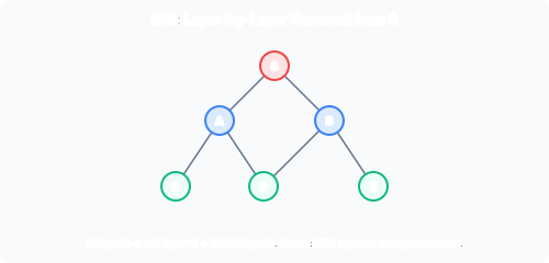
The queue stores the frontier: vertices discovered but whose neighbours have not yet been examined. Because vertices are enqueued in order of discovery (and thus by distance), BFS explores distance $k$ vertices before any distance $k+1$ vertex.

The predecessor array $\pi$ implicitly defines a breadth-first tree: the edges $(v.\pi, v)$ for all $v$ with $v.\pi \neq \text{NIL}$ form a tree rooted at $s$. Following $\pi$ pointers backwards from any vertex reconstructs a shortest path to $s$.

Worked Example

Consider an undirected graph with $V = \{A,B,C,D,E\}$ and edges: $A-B$, $A-C$, $B-D$, $C-D$, $D-E$. Source $s = A$.

Step	Queue	d(A)	d(B)	d(C)	d(D)	d(E)
Init	[A]	0	∞	∞	∞	∞
Deq A	[B,C]	0	1	1	∞	∞
Deq B	[C,D]	0	1	1	2	∞
Deq C	[D]	0	1	1	2	∞
Deq D	[E]	0	1	1	2	3
Deq E	[]	0	1	1	2	3

Predecessor tree: $\pi(B)=A$, $\pi(C)=A$, $\pi(D)=B$ (first visit), $\pi(E)=D$. Shortest path A→E: E→D→B→A (reverse gives A-B-D-E, distance 3).

Complexity Analysis

With adjacency lists: the initialisation loop and the outer while loop touch each vertex once ($\Theta(|V|)$). The inner for loop traverses each edge’s adjacency list entry at most once ($\Theta(|E|)$ for directed, at most $2|E|$ for undirected). Total: $\Theta(|V| + |E|)$.

With adjacency matrix: the inner loop must scan all $|V|$ columns for each dequeued vertex to check if an edge exists. This costs $\Theta(|V|)$ per vertex, giving $O(|V|^2)$ overall. For sparse graphs this is significantly worse.

Key Point: Duplicate Enqueue Prevention

A naive implementation that checks only marked at dequeue time (not at enqueue) can insert the same vertex into the queue multiple times. The GREY/pending flag prevents this: once a vertex is discovered, its colour changes to grey immediately, so subsequent edges to it are ignored.

Summary

Aspect	Detail
Data structure	FIFO queue
Colour scheme	White → Grey → Black
Distance metric	Edge count (unweighted)
Output	$d[v]$ (shortest distance), $\pi[v]$ (predecessor)
Time (adj. lists)	$\Theta(V+E)$
Time (adj. matrix)	$\Theta(V^2)$
Space	$\Theta(V)$ (queue) + $\Theta(V+E)$ (graph)

Past paper questions: y2025p1q9(a)(i) (BFS time bounds with adjacency matrix).