Adjacency Matrix versus Adjacency Lists

Two Standard Representations

There are two fundamental ways to store a graph in memory. The choice of representation directly affects the asymptotic running time of graph algorithms, so understanding the trade-offs is critical for both implementation decisions and exam questions.

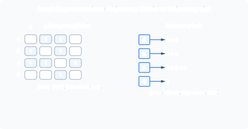
Adjacency Matrix

An adjacency matrix is a $|V| \times |V|$ matrix $M$. For unweighted graphs:

$M[u][v] = \begin{cases} 1 & \text{if } (u, v) \in E \\ 0 & \text{otherwise} \end{cases}$

For weighted graphs, $M[u][v]$ stores the edge weight (and typically $\infty$, 0, or some sentinel for absent edges). For undirected graphs, the matrix is symmetric: $M[u][v] = M[v][u]$. This means only the upper or lower triangle needs to be stored explicitly, roughly halving the memory. For unweighted graphs, each entry can be a single bit.

Space: $\Theta(|V|^2)$ regardless of the number of edges. Even a graph with zero edges allocates a full matrix.

Key operations:

• Test if $(u, v) \in E$: $O(1)$ — single array lookup.
• List all neighbours of vertex $u$: $\Theta(|V|)$ — must scan the entire row $u$.
• Iterate over all edges: $\Theta(|V|^2)$ — must visit every matrix cell.
• Add or remove an edge: $O(1)$ — set or clear a cell.

Adjacency Lists

An array $A$ of length $|V|$, where $A[u]$ points to a linked list or dynamic array containing all $v$ such that $(u, v) \in E$. For weighted graphs, each list entry stores $(v, w(u,v))$.

Space: $\Theta(|V| + |E|)$. Each directed edge contributes one list entry. For undirected graphs, each edge appears in two lists, so space is $\Theta(|V| + 2|E|) = \Theta(|V| + |E|)$.

Key operations:

• Test if $(u, v) \in E$: $O(\deg(u))$ — sequential scan of $u$‘s list. Worst case $O(|V|)$ when $\deg(u) = |V|-1$.
• List neighbours of $u$: $\Theta(\deg(u))$ — exactly the list length.
• Iterate over all edges: $\Theta(|V| + |E|)$ — visit each list head and each entry once.
• Add edge: $O(1)$ (prepend to list). Remove edge: $O(\deg(u))$ (find and delete).
• For undirected graphs, removal must be done from both endpoints’ lists: $O(\deg(u) + \deg(v))$.

Worked Example

Directed weighted graph: $V = \{1, 2, 3, 4\}$, edges $(1,2)$ weight 5, $(1,3)$ weight 2, $(2,4)$ weight 1.

Matrix representation: $\begin{pmatrix} 0 & 5 & 2 & \infty \\ \infty & 0 & \infty & 1 \\ \infty & \infty & 0 & \infty \\ \infty & \infty & \infty & 0 \end{pmatrix}$

Adjacency list representation:

• $A[1] \to (2,5) \to (3,2)$
• $A[2] \to (4,1)$
• $A[3] \to \emptyset$
• $A[4] \to \emptyset$

Space analysis: matrix uses $4 \times 4 = 16$ entries. Lists use 3 list entries + 4 array slot pointers = 7 entries. For this sparse graph ($|E|=3$ of a possible 12), lists are significantly more compact.

Trade-off Summary

Criterion	Adjacency Matrix	Adjacency Lists
Space	$\Theta(V^2)$	$\Theta(V + E)$
Edge query $(u,v)$	$O(1)$	$O(\deg(u)) \le O(V)$
Neighbours of $u$	$\Theta(V)$	$\Theta(\deg(u))$
All edges iteration	$\Theta(V^2)$	$\Theta(V + E)$
Add edge	$O(1)$	$O(1)$
Remove edge	$O(1)$	$O(\deg(u) + \deg(v))$
Best for	Dense graphs	Sparse graphs

Impact on Graph Algorithms

BFS/DFS: With adjacency lists, both run in $\Theta(|V| + |E|)$ because the inner loop visits each neighbour exactly once. With an adjacency matrix, the inner loop must scan all $|V|$ columns for each dequeued/extracted vertex, costing $\Theta(|V|)$ per vertex. Total: $O(|V|^2)$ regardless of edge count.

Exam point (y2025p1q9): Tight bounds for BFS with adjacency matrix are $\Omega(|V|^2)$ and $O(|V|^2)$; with lists, $\Omega(|V|+|E|)$ and $O(|V|+|E|)$.

Dijkstra: With binary heap and adjacency lists: $O((|V|+|E|)\log |V|)$. With matrix: neighbour iteration becomes $\Theta(|V|)$ per vertex, and using a simple array instead of heap gives $O(|V|^2)$, which can be faster than $O(|V|^2 \log |V|)$ for dense graphs due to lower constants.

Floyd-Warshall: Inherently uses a matrix (the distance matrix itself), running in $\Theta(|V|^3)$. Johnson’s algorithm relies on adjacency lists for sparsely efficient Dijkstra calls.

Summary

Property	Matrix	Lists
Space	$\Theta(V^2)$	$\Theta(V+E)$
Edge test	$O(1)$	$O(V)$ worst
Neighbour listing	$\Theta(V)$	$\Theta(\deg(v))$
BFS/DFS time	$O(V^2)$	$\Theta(V+E)$
Use when	$E = \Theta(V^2)$	$E = O(V)$

Past paper questions: y2025p1q9(a)(i) (BFS complexity bounds with adjacency matrix).