Kosaraju's Algorithm

Overview

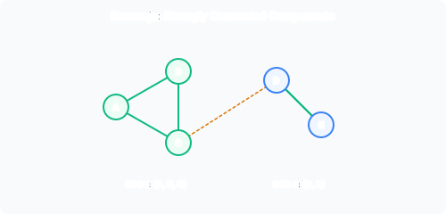
Kosaraju’s algorithm finds all strongly connected components (SCCs) of a directed graph in $\Theta(|V| + |E|)$ time using two complete passes of DFS. It is elegant and requires only basic DFS, making it a natural exam topic.

Algorithm: Three Steps

1. DFS on $G$: Run a full DFS on the original graph $G$. Record the finish time $f[v]$ for every vertex.
2. Transpose: Compute the transpose graph $G^T$: reverse the direction of every edge. $V^T = V$, $E^T = \{(v,u) \mid (u,v) \in E\}$.
3. DFS on $G^T$: Run DFS on $G^T$, but in the outer loop (which picks the next root), process vertices in decreasing order of their finish times from step 1. Each DFS tree in this forest is one SCC of $G$.

Pseudocode

KOSARAJU(G):
  // Step 1: DFS on G, record finish times
  for each v in G.V:
    v.colour = WHITE
    v.π = NIL
  time = 0
  order = []                 // list for finish-time ordering
  for each v in G.V:
    if v.colour == WHITE:
      DFS-VISIT-FINISH(G, v, order)

  // Step 2: Compute G^T
  GT = TRANSPOSE(G)

  // Step 3: DFS on G^T in reverse finish order
  for each v in GT.V:
    v.colour = WHITE
  sccs = []
  for each v in reverse(order):  // decreasing finish time
    if v.colour == WHITE:
      component = []
      DFS-VISIT-COLLECT(GT, v, component)
      sccs.append(component)
  return sccs

Intuition

Why does processing $G^T$ in decreasing finish-time order produce SCCs?

• In step 1, DFS on $G$ assigns finish times. The SCC that acts as a sink in the component DAG (no outgoing edges to other SCCs) finishes first amongst its DFS tree. More generally, finish times reveal the topological order of the component DAG: components earlier in the topological order finish later.
• In step 3, we reverse all edges. The sink SCC in $G$ becomes a source SCC in $G^T$. Since we process vertices in decreasing finish order, we start DFS from a vertex in the “last-finishing” component (a sink in $G$, source in $G^T$). Because edges between SCCs are reversed, the DFS cannot escape this SCC into others that haven’t been visited yet.
• Within an SCC, edges go both ways, so reversing preserves strong connectivity: if vertices $u$ and $v$ are mutually reachable in $G$, they remain mutually reachable in $G^T$.

Worked Example

Graph with $V = \{1,2,3,4,5,6,7,8\}$ and edges (as in the SCC notes):

$1 \to 2$, $2 \to 3$, $2 \to 4$, $3 \to 1$, $3 \to 4$, $4 \to 3$, $5 \to 4$, $5 \to 6$, $6 \to 5$, $6 \to 7$, $7 \to 8$, $8 \to 6$, $8 \to 7$.

Step 1: DFS on $G$, start at 1 (assume adjacency list order as listed). Discovery/finish times:

Vertex	1	2	3	4	5	6	7	8
$d$	1	2	3	4	12	13	8	5
$f$	16	15	10	7	11	14	9	6

(Values depend on adjacency order; any valid DFS is fine.) Decreasing finish order: $1, 2, 6, 5, 3, 7, 4, 8$.

Step 2: $G^T$. All edges reversed: $2 \to 1$, $3 \to 2$, $4 \to 2$, $1 \to 3$, $4 \to 3$, $3 \to 4$, $4 \to 5$, $6 \to 5$, $5 \to 6$, $7 \to 6$, $8 \to 7$, $6 \to 8$, $7 \to 8$.

Step 3: DFS on $G^T$, order: 1, 2, 6, 5, 3, 7, 4, 8.

• Start from 1 (first in order). DFS from 1 reaches $\{1,3,4,2\}$. This is SCC $\{1,2,3,4\}$.
• Next unvisited in order: 6. DFS from 6 reaches $\{6,5,8,7\}$. This is SCC $\{5,6,7,8\}$.
• Result: two SCCs as expected.

Time Complexity

• DFS on $G$: $\Theta(|V| + |E|)$.
• Computing $G^T$: $\Theta(|V| + |E|)$ (reverse every edge).
• DFS on $G^T$: $\Theta(|V| + |E|)$.
• Total: $\Theta(|V| + |E|)$ — linear in the size of the graph.

The algorithm is optimal: any algorithm must at least examine every vertex and edge to find all SCCs.

Correctness Sketch

Let $C_1$ and $C_2$ be two distinct SCCs of $G$ with an edge from $C_1$ to $C_2$ in the component DAG. In step 1, all vertices in $C_1$ finish after all vertices in $C_2$, assuming $C_1$ is explored first. More formally, the finish-time ordering corresponds to a reverse topological sort of the component DAG. Thus, when we process $G^T$ in decreasing finish order, we first explore a sink SCC of $G$ (now a source in $G^T$), and edges to other SCCs point the opposite way in $G^T$, so the DFS stays within the current SCC. The official proof is in CLRS Chapter 22.

Summary

Step	Action	Time
1	DFS on $G$, record $f[v]$	$\Theta(V+E)$
2	Construct $G^T$	$\Theta(V+E)$
3	DFS on $G^T$, decreasing $f[v]$ order	$\Theta(V+E)$
Total		$\Theta(V+E)$

Past paper questions: SCCs are assessed conceptually; Kosaraju’s algorithm may appear as a direct algorithm question or as part of a larger problem.