Operating Systems

The extended machine

An operating system is a layer of software that sits between the hardware and the application programs. It presents the hardware to programmers through a cleaner, more convenient interface — the extended machine (or virtual machine) metaphor.

The raw hardware provides registers, memory addresses, and I/O ports. The OS wraps these in abstractions:

Programmers write to these abstractions, not to the bare metal. If the hardware changes, only the OS needs to adapt; the application interface stays stable.

The resource manager

The OS also acts as a resource manager, arbitrating competing demands for the machine’s physical resources. It decides:

• Which process runs on the CPU and for how long
• Which regions of memory are allocated to which process
• Who can read or write a file
• Which disk blocks belong to which file

In a multi-user, multi-process system, the OS provides multiplexing (sharing resources in time or space) and protection (preventing interference between processes).

Kernel and user mode

To enforce protection, the CPU provides at least two privilege levels:

• Kernel mode (supervisor mode): can execute all instructions, including privileged ones like I/O operations and page table manipulation.
• User mode: restricted; attempts to execute privileged instructions cause a trap into the kernel.

The OS kernel runs in kernel mode; user programs and most services run in user mode. The boundary between them is the system-call interface.

System calls

A system call is how a user program requests a service from the kernel — opening a file, reading data, spawning a process, sending a signal. The sequence is:

1. Program puts arguments in registers (or on the stack).
2. Program executes a special trap instruction (e.g., syscall on x86-64, svc on ARM).
3. CPU switches to kernel mode and jumps to a predefined kernel entry point.
4. Kernel validates arguments, performs the operation, and returns a result.
5. CPU returns to user mode at the instruction after the trap.

System calls are expensive compared to ordinary function calls (context switch overhead), but they are the only gateway into the kernel.

Summary

• The OS is both an extended machine (providing clean abstractions) and a resource manager (arbitrating hardware).
• Hardware-enforced dual-mode operation separates user code from kernel code.
• System calls are the controlled entry point from user mode into the kernel.

Past Paper Questions

2019 Paper 2 Question 4(a): Describe the mechanisms by which an operating system protects a user process’ use of system resources (CPU, memory, I/O) from accidental or deliberate interference. Indicate what special hardware is required. [6 marks]

Monolithic kernels

Most general-purpose operating systems — including Linux, the BSDs, and Windows — use a monolithic kernel architecture. The entire kernel runs in a single address space in kernel mode. All kernel services (scheduling, memory management, file systems, networking, device drivers) live inside this space and can call each other directly.

Advantages:

• Fast cross-component calls (simple function calls, no IPC overhead).
• Straightforward to implement initially.
• Good performance for tightly-coupled subsystems.

Disadvantages:

• A bug in any component (e.g., a device driver) can crash the whole kernel.
• Large codebase; harder to verify correctness.
• Adding or updating components often requires rebuilding and rebooting (though Linux kernel modules mitigate this somewhat).

Microkernels

A microkernel strips the kernel down to the bare minimum — typically address spaces, threads, and inter-process communication (IPC) — and runs everything else (file systems, networking, device drivers) in user-mode server processes.

Examples: MINIX, L4, seL4, QNX, the GNU Hurd.

Advantages:

• A crash in a file-system server does not bring down the kernel.
• Servers can be started, stopped, and updated independently.
• Smaller trusted computing base (TCB) — easier to verify formally.

Disadvantages:

• Cross-component communication goes through IPC, which is slower than direct function calls.
• Real-world microkernels often bring key servers back into kernel space for performance, blurring the distinction.

Hybrid kernels

Most modern desktop OSes (Windows NT, macOS XNU) are hybrid kernels: they retain a monolithic core but run some services (e.g., graphics, USB) in user mode. The goal is to get microkernel-like modularity without paying the full IPC cost. Linux is sometimes described as hybrid when kernel modules are loaded, but its core architecture is monolithic.

Unikernels

A unikernel compiles the application and the minimal OS library into a single address space that runs directly on the hypervisor. There is no user/kernel split — everything runs at the highest privilege. Unikernels are used for cloud workloads where a full OS would be overhead.

Example: MirageOS (OCaml).

Exokernels

An exokernel takes the opposite approach: instead of abstracting hardware away, it securely multiplexes it, giving each application a raw slice (disk blocks, physical memory frames, network rings). The application’s own library OS decides how to use them. This gives applications maximum control at the cost of making them more complex.

OS components (monolithic view)

Regardless of architecture, every general-purpose OS contains:

Summary

• Monolithic kernels (Linux, BSDs) are fast but fragile.
• Microkernels (L4, seL4) are robust but pay IPC costs.
• Real-world systems are often hybrids.
• Exokernels and unikernels represent opposing extremes on the abstraction-control spectrum.

The system-call interface

A system call provides the controlled gateway from user space into the kernel. Each call is identified by a number (e.g., on x86-64 Linux: write = 1, open = 2, close = 3, fork = 57). The user program puts the system-call number and arguments in designated registers, then invokes the trap instruction.

The trap flow

1. User space preparation: The C library (libc) wraps the system call in a function. The wrapper places the syscall number in rax (x86-64) or x8 (ARM64), places up to six arguments in registers (rdi, rsi, rdx, r10, r8, r9 on x86-64), and issues the trap instruction (syscall).

2. Hardware trap: The CPU atomically:

   • Switches the privilege level from user to kernel.
   • Saves the current program counter and stack pointer into kernel-controlled registers.
   • Jumps to a kernel entry point defined at boot time (e.g., entry_SYSCALL_64 in Linux).
   • Switches to the kernel stack.

3. Kernel dispatching: The kernel entry code saves all general-purpose registers onto the kernel stack (preserving the user context), then uses the syscall number in rax to index into the system-call table. Each entry is a function pointer. The kernel calls the appropriate handler (e.g., __x64_sys_write).

4. Execution: The handler validates arguments (checking pointers belong to the calling process and do not point into kernel memory), then performs the operation.

5. Return: The kernel restores user registers from the saved state on the kernel stack, executes a return-from-interrupt instruction (sysret on x86-64, eret on ARM64), and the CPU atomically switches back to user mode.

Cost of a system call

A system call is orders of magnitude more expensive than a user-space function call because:

• The trap instruction flushes the pipeline and incurs a branch-prediction penalty.
• The kernel must save and restore dozens of registers.
• Cache state is disturbed — kernel code and data displace user cache lines.
• Argument validation adds overhead (especially for pointer-heavy calls).
• On return, TLB entries may need to be reloaded.

Historically, early Linux system calls cost hundreds of cycles; modern mitigations (e.g., KPTI for Meltdown) have made them more expensive again, sometimes exceeding a thousand cycles.

Classes of system calls

Summary

• System calls are numbered, dispatched through a trap-instruction → kernel-entry → syscall-table path.
• The trap instruction is the only way to cross from user into kernel mode.
• Syscall overhead is significant (hundreds to thousands of cycles) but unavoidable.
• The kernel must validate every argument to prevent user code from corrupting or reading kernel memory.

Three control-transfer mechanisms

The CPU transfers control to the kernel through three mechanisms, all of which ultimately lead to a kernel entry point via the interrupt descriptor table (IDT):

Interrupts are asynchronous — they are not caused by the currently running instruction. Traps and exceptions are synchronous — they are caused by the current instruction.

Interrupts in detail

An interrupt is a hardware signal that arrives on one of the CPU’s interrupt pins. The CPU checks for pending interrupts at the boundary between instructions (or at interruptible points during long instructions).

When an interrupt is accepted:

1. The CPU finishes the current instruction (or reaches an interruptible point).
2. It pushes the current program counter, the stack pointer, and the flags register onto the kernel stack.
3. It reads the interrupt vector from the interrupting device (or the interrupt controller, e.g., APIC).
4. It indexes the IDT with this vector to find the address of the Interrupt Service Routine (ISR).
5. It jumps to the ISR in kernel mode.

The ISR does the minimum possible work (acknowledge the interrupt, copy data from device registers, schedule a deferred bottom half) and returns. Interrupts remain disabled for the duration of the ISR unless the ISR explicitly re-enables them — long ISRs cause lost interrupts.

Exceptions in detail

An exception is the CPU’s response to a fault during instruction execution:

The interrupt-descriptor table (IDT)

The IDT is an array of 256 gate descriptors set up by the OS at boot time. Each entry specifies:

• The address (segment selector + offset) of the handler.
• The privilege level required to invoke it (some gates, like int3, are callable from user mode; most are kernel-only).
• The gate type (interrupt gate disables further interrupts; trap gate does not).

The LIDT instruction tells the CPU where the IDT lives.

Software interrupts and int instruction

The x86 int n instruction triggers a software interrupt. Historically, Linux used int 0x80 for system calls. This instruction is slower than syscall/sysenter (introduced with Pentium II/Athlon) because int must perform ring- and stack-switching logic in microcode. Modern kernels use syscall (x86-64) or sysenter (x86-32) for system calls, but int remains used for traps like breakpoints (int3).

Summary

• Interrupts are hardware-driven and asynchronous; traps and exceptions are software-driven and synchronous.
• All three use the IDT to vector to kernel handlers.
• ISRs must be short — defer work to bottom halves or kernel threads.
• Faults (like page faults) are fixable; aborts are not.
• syscall is the modern fast system-call mechanism, superseding the older int 0x80.

The mode bit

The CPU provides at least two execution privilege levels, distinguished by a mode bit in a processor status register (e.g., the Current Privilege Level, CPL, in x86’s CS register):

• Kernel mode (mode bit = 0): the CPU can execute privileged instructions — halt, modify the page table, access I/O ports, mask interrupts.
• User mode (mode bit = 1): privileged instructions cause an exception (a trap into the kernel).

The kernel itself runs in kernel mode. Every user process — including system daemons — runs in user mode. The mode bit ensures that user code cannot accidentally or maliciously damage the system.

Privileged instructions

Which instructions are privileged varies by architecture. Examples on x86-64:

Attempting a privileged instruction in user mode raises a general protection fault (#GP), which vectors into the kernel’s exception handler. The kernel typically terminates the offending process with SIGILL or SIGSEGV.

Transition: user → kernel

The only way into kernel mode from user mode is through a controlled hardware mechanism — a trap, an interrupt, or an exception. The CPU atomically:

1. Switches the privilege level to kernel.
2. Saves the current program counter, stack pointer, and flags.
3. Jumps to a kernel-controlled handler address (from the IDT or a model-specific register).

The user process cannot choose the kernel code that runs — it can only supply a system-call number. The kernel demultiplexes and validates it.

Transition: kernel → user

Returning to user mode is explicit. The kernel executes a return-from-interrupt instruction (sysret, iretq, eret), which atomically:

1. Restores the user-mode stack pointer and program counter from saved kernel-stack state.
2. Switches the privilege level back to user.
3. Resumes execution at the saved instruction address.

Why not a single mode?

Early single-user OSes (MS-DOS, classic Mac OS) ran everything at the highest privilege. A crashed application could overwrite the OS, corrupt the disk, or hang the machine. Modern systems use dual-mode (or more — e.g., x86 has four rings, though most OSes use only rings 0 and 3) to provide isolation: a user process can crash itself without taking down the system.

Summary

• The mode bit prevents user code from executing privileged instructions.
• Traps, interrupts, and exceptions are the only controlled entries into kernel mode.
• The kernel must never trust user-supplied arguments without validation — the user could be malicious.

Past Paper Questions

2019 Paper 2 Question 4(a): Describe the mechanisms by which an OS protects a user process’ use of system resources from interference by other processes. Indicate what special hardware is required. [6 marks]

The problem

Without memory protection, Process A could write to addresses belonging to Process B (or the kernel), corrupting data, stealing information, or crashing the system. The OS must enforce address-space isolation: each process can only access its own memory.

Base and limit registers

The simplest hardware mechanism uses two registers:

• Base register: the smallest physical address that the process may access.
• Limit register: the size of the process’s legal address range.

On every memory access, the hardware (typically the MMU) checks:

$\text{base} \le \text{address} < \text{base} + \text{limit}$

If the check fails, the MMU raises an exception (a segmentation fault), and the kernel terminates the offending process.

The base and limit registers are kernel-mode-only — the MOV instructions that modify them are privileged. On a context switch, the kernel saves the outgoing process’s base and limit and loads the incoming process’s values, thereby switching the protected address space.

Logical-to-physical translation

With base-and-limit hardware, every address a process uses is logical (or virtual). The hardware adds the base register to every address before sending it to the memory bus:

$\text{physical address} = \text{base} + \text{logical address}$

Process A’s logical address 0 maps to physical address base_A; Process B’s logical address 0 maps to base_B. Each process sees a contiguous address space starting at zero.

Limitations

Base-and-limit protection is simple but inflexible:

• No growth: a process that needs more memory than limit must be killed, moved, or resized — all expensive.
• Contiguous allocation: the entire address space must be one contiguous block of physical memory, leading to external fragmentation.
• No sharing: two processes cannot share a subset of pages (e.g., shared libraries) without overlapping the entire segment.
• No sparse addressing: the entire limit region must be backed by physical memory, even if the process uses only scattered pages.

Evolution

Base-and-limit was used in early systems (e.g., the CDC 6600). Modern architectures use paging (see [/modules/os/05-paging-and-page-tables/](managing memory)) which provides per-page protection, sparsity, and sharing — at the cost of more complex hardware.

However, the conceptual model persists: every process has its own address space, and the hardware checks every access against a kernel-managed configuration before allowing it.

Summary

• Base and limit registers enforce per-process memory isolation with a simple bounds check on every access.
• The MMU translates logical addresses by adding the base register.
• The scheme requires contiguous physical allocation and cannot support sparse address spaces or fine-grained sharing.
• Modern systems use paging, which generalises the idea: instead of one base-limit pair, there is a page table with per-page protection.

What it represents

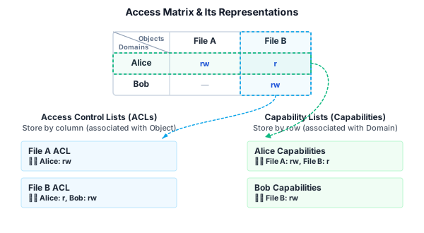
The access matrix is an abstract model of protection. Rows are domains (subjects, principals — users or processes). Columns are objects (files, devices, processes, memory segments). Each cell specifies the access rights the domain has over the object — typically read, write, execute, or owner.

The matrix is sparse: most domains have no rights over most objects. A modern system with thousands of users and millions of files wastes space if the full matrix is stored literally.

Two concrete representations

Access Control Lists (ACLs)

Store the matrix by column — each object carries a list of (domain, rights) pairs. When a domain tries to access an object, the OS checks whether that domain appears in the object’s ACL and whether the requested right is granted.

Examples: UNIX file permissions (simplified ACL — three fixed domains: owner, group, other), Windows NTFS ACLs (fully general: arbitrary users and groups with arbitrary rights), AWS S3 bucket policies.

Advantages:

• Easy to revoke: change the object’s ACL and it takes effect immediately.
• The object’s owner controls access directly.
• Natural for most access patterns (many users, many files — attach access to the file).

Disadvantages:

• Checking access requires scanning the list (though caching mitigates this).
• Delegation is awkward: to delegate a file right, the owner must modify the ACL.

Capabilities

Store the matrix by row — each domain holds a set of capabilities, where a capability is an unforgeable token representing a specific right to a specific object. The domain presents the capability as a “key” or “ticket” when accessing the object.

Examples: UNIX file descriptors (once a file is opened, the process holds a capability-like descriptor; closing it destroys the capability), Hydra, KeyKOS, CHERI hardware capabilities.

Advantages:

• Natural delegation: passing a capability to another domain is straightforward (if the OS supports it).
• No need to scan an ACL on every access — possession of the capability proves the right.
• Fine-grained: a capability can grant one specific right (read-only) without implying others.

Disadvantages:

• Revocation is hard: if Alice passed a capability to Bob, taking it back requires revoking all capabilities that derive from the original, which can cascade.
• A domain may accumulate a large number of capabilities.

UNIX hybrid approach

UNIX uses a pragmatic hybrid:

• ACLs for file access at open() time: the kernel checks the owner/group/other permission bits against the process’s UID and GID.
• Capabilities for open files: the returned file descriptor is unforgeable by the process (it’s just an integer index into the kernel’s per-process file table) and can be passed to fork()-ed children or across UNIX-domain sockets via SCM_RIGHTS.

Which to use?

On a modern personal laptop, ACLs make more sense: a small number of users but a very large number of files. Each user carries membership in a handful of groups, and files grant access to those groups. Capabilities would require every user to carry an enormous set of capabilities — one per accessible file — which is impractical for POSIX file systems.

Past Paper Questions

2025 Paper 2 Question 3(a): The access matrix may be very large but also very sparse. State the two common representations of the access matrix, and explain which you would use to represent access rights for a modern personal laptop. [4 marks]

2019 Paper 2 Question 4(c): Describe how you might implement a capability system to protect files from access, give a possible API, and compare your proposal to the UNIX access control method. [8 marks]

The 9-bit permission model

UNIX file permissions use a simplified ACL scheme with three fixed domains:

Each file has a 9-bit permission mask, typically displayed as rwxrwxrwx (user/group/other). The kernel stores these bits in the file’s inode.

Octal representation

Permissions are commonly given in octal, where r = 4, w = 2, x = 1:

So chmod 640 file means: owner rw- (6), group r-- (4), other --- (0).

Special permission bits

SetUID is a powerful (and dangerous) mechanism: a SetUID root programme runs with full kernel privileges. Vulnerabilities in SetUID programmes are a classic privilege-escalation vector.

Access check algorithm

When process P tries to open file F for operation O:

1. If P’s effective UID is 0 (root), access is granted unconditionally (unless the file system is mounted noexec or read-only, or the file is on NFS with root_squash).
2. If P’s effective UID equals F’s owner UID, the owner permission bits are checked.
3. Else, if P’s effective GID (or any supplementary group) equals F’s group GID, the group permission bits are checked.
4. Else, the other permission bits are checked.

For directories, r permits listing, w permits creating/deleting entries, and x permits traversal (using the directory in a path).

The open-time check

UNIX checks permissions at open() time, not at each read() or write(). The returned file descriptor acts as a capability — once obtained, the process can use it until close() even if the file’s permissions are subsequently changed. This is efficient (check once, use many times) but means a process can retain access to a file whose permissions have been revoked, as long as it does not close and reopen the descriptor.

Performing the check on every read()/write() would be safer but more expensive, and would require handling the case where a descriptor becomes invalid mid-operation.

The root user

UID 0 (root) bypasses all permission checks. This is a convention implemented in the kernel, not a property of the permission bits. The username “root” is just a mapping in /etc/passwd; what matters is UID 0. If you change root’s UID to 1000, processes running under that UID lose special privileges, and the old UID 0 (now unnamed in /etc/passwd) retains them.

Past Paper Questions

2025 Paper 2 Question 3(c): Describe how an administrator might configure users, groups and file permissions to create files with specific permission patterns. [7 marks]

2025 Paper 2 Question 3(d): What happens if root’s UID is changed from 0 to 1000? [4 marks]

Question format

Tripos questions often ask you to construct an access matrix from a set of natural-language policy statements. The process is mechanical but requires care: identify all domains (subjects), all objects, and the allowed operations for each (domain, object) pair.

Worked example: 2025 Paper 2 Question 3(b)

Three user accounts (alice, bob, chris) plus root. Four peripherals: printer, removable hard disk, web camera with microphone, speakers. Policy:

1. Alice may use the printer fully; Chris may not use the printer at all; Bob may only check the printer’s status.
2. Only root may create backups; only Bob may recover files from a backup.
3. Alice and Bob may participate fully in video-conferences; Chris may only play music.

Step-by-step:

Step 1: Identify domains and objects

Domains: root, alice, bob, chris. Objects: Printer, Hard disk, Web camera, Speaker.

Step 2: Root gets everything

Root is the superuser. In any UNIX-derived access matrix, root has read/write on every object by default. (Mark scheme: marks lost for not granting root full permissions.)

Step 3: Translate each policy statement

Printer:

• Alice: full use → read/write (can both submit and check status).
• Bob: check status only → read (can read status but not submit jobs).
• Chris: no access → —.

Hard disk (backups):

• Root: create backups → read/write.
• Alice: policy says nothing → —.
• Bob: recover files → read (can read from backups but not write them).
• Chris: policy says nothing → —.

Web camera (video-conferences):

• Root: read/write.
• Alice: full video-conferencing → read (receive video) — and actually she needs write too (transmit). Wait: the natural interpretation of “participate fully” for a camera is that the camera provides video input — and for video-conferencing, the system must both capture (read) and transmit (arguably write). The mark scheme grants read for alice and bob on the camera.
• Bob: same as alice → read.
• Chris: music only — no video → —.

Speaker:

• Root: read/write.
• Alice: full participation — can output audio → write.
• Bob: same → write.
• Chris: play music → write (but not read — reading a speaker makes no physical sense).

Step 4: Construct the matrix

Common mistakes

• Inventing non-standard operations beyond read and write.
• Forgetting that root has automatic read/write on everything.
• Assigning permissions that don’t make physical sense (e.g., read on a speaker — what would you “read” from a speaker?).
• Treating “web camera” as two separate objects when the question groups them. Read the object list carefully.

Summary

• Identify domains, objects, and the two operations (read, write).
• Root gets read/write on everything.
• Translate each policy sentence mechanically to read, write, or —.
• Avoid invented operations and physically nonsensical permissions.

UID and GID

Every UNIX process carries two user identifiers and two group identifiers:

Additionally, a process may have a list of supplementary GIDs (groups the user is a member of). Permission checks test the effective UID and all effective GIDs (primary + supplementary).

The kernel cares about numbers, not names

The kernel identifies users and groups by integer IDs, not string names. The root user is UID 0; this privilege is hard-coded in the kernel — any process with effective UID 0 bypasses permission checks and can execute privileged instructions via system calls.

The mapping between names and numbers lives in user-space databases: /etc/passwd (users) and /etc/group (groups). The kernel never reads these files; user-space utilities (login, id, ls -l) consult them to display human-readable names.

A critical Tripos insight: changing root’s UID from 0 to 1000 in /etc/passwd means the name “root” maps to UID 1000, and UID 0 is now unnamed. The access matrix does not change — UID 0 still has all permissions. But logging in as “root” now gives you UID 1000, which has no special privileges. Administration becomes nearly impossible unless sudo or another mechanism is available.

Groups

A UNIX user belongs to one primary group (recorded in /etc/passwd) and zero or more supplementary groups (recorded in /etc/group). Each file has one owning user and one owning group.

Groups are the mechanism for sharing beyond the owner. If you want Alice and Charlie (but not others) to read a file, you create a group alice_charlie and assign the file to that group with g=r--.

Only one group can be associated with a given file at a time. For more complex sharing, use ACLs (POSIX ACLs extend the traditional 9-bit model with setfacl/getfacl).

Creating permission patterns (Tripos style)

Given a required permission pattern, the administrator must decide ownership and group membership:

Pattern 1: readable and writable by root and alice, readable by bob.

• Create group gbob = {bob}.
• File ArwBr owned by alice, group gbob, permissions u=rw, g=r, o= → 640.
• Or: owned by bob, group galice, u=r, g=rw, o= → 460.

Pattern 2: readable and writable by root and bob, readable by any user.

• File owned by bob, any group, permissions u=rw, g=r, o=r → 644.
• Or: owned by anyone, group gbob, permissions g=rw, o=r → 064.

Pattern 3: owned by alice but readable and writable only by root.

• File owned by alice, any group, permissions 000.
• Root bypasses permissions and can read/write; alice owns it but cannot access it (permissions deny even the owner). Alice can chmod it back since she owns it.

Summary

• The kernel uses numeric UID/GID; names are user-space conventions.
• UID 0 = root privilege is hard-coded; changing the name’s mapping does not change the privilege.
• Groups enable sharing; each file has exactly one group.
• Permission patterns on Tripos questions are constructed by choosing ownership, group membership, and a 9-bit permission mask.

Process vs programme

A programme is a passive entity — an executable file stored on disk (e.g., /bin/ls). A process is an active entity — a programme in execution, with a current program counter, a stack, a heap, and an entry in the kernel’s process table.

A single programme can be executing in multiple processes simultaneously (e.g., several terminal windows each running a shell). Each process has its own independent state.

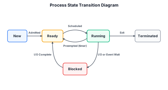
The five-state model

A process moves through states during its lifetime:

Transitions:

• New → Ready: The kernel admits the process to the scheduling system.
• Ready → Running: The scheduler selects the process and dispatches it.
• Running → Ready: The scheduler pre-empts the process (timer interrupt) to give another process CPU time.
• Running → Blocked: The process makes an I/O request or waits for a signal.
• Blocked → Ready: The awaited event completes.
• Running → Terminated: The process calls exit() or is killed by a signal.

The Process Control Block (PCB)

The PCB is the kernel’s per-process data structure. It contains everything the kernel needs to manage and suspend/resume the process:

The collection of all PCBs (the process table) is a fixed-size kernel array. On Linux, it’s small — a few hundred entries — because each entry is a task_struct (over 1 KB). The process table size limits the maximum number of processes.

Context switch

When the kernel switches the CPU from Process A to Process B:

1. A trap or interrupt enters the kernel (e.g., timer interrupt, or A makes a blocking system call).
2. The kernel saves A’s registers, program counter, and stack pointer into A’s PCB.
3. The kernel selects B as the next process to run (the scheduler’s job).
4. The kernel restores B’s registers, program counter, and stack pointer from B’s PCB.
5. The kernel returns to user mode, and B resumes where it was suspended.

Context switches are pure overhead: while switching, the CPU does no useful work for any process. Typical context-switch times are on the order of microseconds, but frequent switches degrade throughput.

The process tree

In UNIX, every process (except init/PID 1) is created by fork() from a parent. This forms a tree. When a process terminates, the kernel sends SIGCHLD to its parent and retains the terminated process’s PCB as a zombie until the parent calls wait(). If the parent exits first, the orphan is reparented to init, which reaps zombies.

Summary

• A programme is static; a process is dynamic.
• Processes move through five states; the kernel manages transitions.
• The PCB contains all state needed to suspend and resume a process.
• Context switching saves and restores processor state; it is overhead, not useful work.

PCB contents in detail

The PCB is the kernel’s representation of a process. On Linux, it is the task_struct — one of the largest kernel structures. The key fields relevant to the Tripos:

Processor state area

• General-purpose registers: rax, rbx, rcx, …, r15 (x86-64). Must be saved so the process can resume mid-computation.
• Program counter (rip on x86-64): address of the next instruction.
• Stack pointer (rsp): top of the user-mode stack.
• Frame pointer (rbp): base of the current stack frame.
• Flags register (rflags): condition codes, interrupt-enable bit, mode bit.
• Floating-point / SIMD state: SSE/AVX registers are large and expensive to save; the kernel often saves them lazily (only on first use by the new process).

Memory management

• Page table base (CR3 register value): the root of the process’s page-table tree. Reloading CR3 flushes all TLB entries not tagged with a process ID (on hardware that supports PCIDs, the flush is partial).
• Memory map (mm_struct): describes all mapped regions (text, data, heap, stack, mmap files) with their virtual addresses and permissions.

File and I/O state

• File descriptor table: an array indexed by the small integers returned from open(). Each entry points to a kernel file object.
• Current working directory: the cwd entry in the file descriptor table.

Scheduling and accounting

• Policy and priority: which scheduling class (CFS, real-time, idle), static priority, and nice value.
• Runtime statistics: accumulated virtual runtime (vruntime), recent CPU utilisation (decayed exponentially).
• Timers: the sum of time spent in user mode and in kernel mode, tracked for profiling and for the alarm system call.

Context-switch steps

A full context switch from Process A to Process B:

1. Trap/interrupt: CPU enters kernel mode. The hardware saves the user-mode rip, rsp, and rflags onto the kernel stack.
2. Save A’s state: The kernel’s trap-entry assembly saves the remaining user-visible registers (general-purpose, segment registers) onto the kernel stack, then saves the kernel stack pointer into A’s task_struct.
3. Scheduler: Calls pick_next_task(), which selects B (based on CFS vruntime, priority, etc.).
4. Switch address space: Loads B’s page table by writing the physical address of B’s top-level page table into CR3. (On hardware with PCID, the TLB flush is selective.)
5. Restore B’s state: Loads B’s kernel stack pointer from B’s task_struct, pops the saved registers from B’s kernel stack, and returns to user mode — which restores rip, rsp, and rflags atomically.
6. B resumes: The CPU is now executing B at whatever instruction was next in B’s saved rip.

Cost factors

Millisecond-scale context switches would be catastrophic. Realistic figures are 1–10 µs, but the dominant cost is usually the post-switch cache and TLB warming, not the switch itself.

Summary

• The PCB stores all processor state, memory mappings, file descriptors, and scheduling parameters.
• Context switching saves A’s state, selects B, switches address spaces, and restores B’s state.
• The big costs are TLB flushes and cache displacement, not register save/restore.

Overview

UNIX creates new processes through two system calls:

• fork(): creates an exact child copy of the calling process. The child inherits the parent’s memory, file descriptors, and execution context.
• execve(): replaces the calling process’s address space with a new programme loaded from disk. The PID, file descriptors, and environment survive; everything else is replaced.

Together, fork + exec is the standard pattern: the shell forks, and the child execs the desired command.

fork() in detail

pid_t fork(void);

fork() returns twice — once in the parent (returning the child’s PID) and once in the child (returning 0). This is the fundamental UNIX idiom; every process (except PID 1) was created by fork().

The kernel must duplicate:

The child gets a new, unique PID. The parent-child relationship is recorded in the process tree.

Copy-on-write efficiency

Naively copying the entire address space (potentially gigabytes) on every fork() would be ruinous. COW avoids this:

1. During fork(), the kernel marks all pages in both parent and child as read-only.
2. No physical copy is made — both processes read from the same physical frames.
3. When either process attempts a write, the MMU raises a page fault (protection fault — writing a read-only page).
4. The page-fault handler sees that the page is a COW page. It allocates a new physical frame, copies the page’s data, updates the faulting process’s page table to point to the new frame (now read-write), and retries the faulting instruction.
5. The other process continues to share the original frame (also now marked read-write again if the writer was the only other sharer).

The common fork()-immediately-exec() case is optimised further: exec() will replace the entire address space anyway, so copying is entirely wasted. Modern kernels use vfork() or clone() with flags that avoid even the COW setup.

execve() in detail

int execve(const char *pathname, char *const argv[], char *const envp[]);

If successful, execve() does not return — the calling process is replaced. The old address space is discarded; the kernel:

1. Validates that the file at pathname exists, is executable, and the caller has execute permission.
2. Optionally, if the file has a SetUID or SetGID bit, changes the process’s effective UID/GID.
3. Loads the executable’s segments into memory (text at the virtual address specified by the ELF headers, data, BSS).
4. Sets up a new stack with the argv and envp strings, and auxiliary vectors.
5. Sets the program counter to the executable’s entry point.

File descriptors survive exec() unless they were opened with the FD_CLOEXEC flag. This allows the shell to set up pipes and redirections before the child execs — the child inherits the file descriptors and uses them transparently.

The fork–exec pattern

pid_t pid = fork();
if (pid == 0) {
    // Child
    close(pipefd[0]);          // close read end
    dup2(pipefd[1], STDOUT_FILENO);
    execlp("ls", "ls", "-l", NULL);
    // execlp never returns on success
    perror("exec failed");
    _exit(1);
} else {
    // Parent
    close(pipefd[1]);          // close write end
    wait(NULL);                 // reap the child
}

Summary

• fork() duplicates the process; exec() replaces the programme.
• Copy-on-write makes fork() cheap — no physical copy of memory until a write occurs.
• File descriptors survive exec(), enabling I/O redirection.
• The shell’s job is to fork, set up pipes and redirections, and exec the command.

What a scheduler does

The scheduler (or dispatcher) selects which of the ready processes runs next on the CPU. It is invoked whenever:

• A process transitions from Running → Blocked (non-preemptive yield).
• A process transitions from Running → Ready (timer interrupt — preemption).
• A process transitions from Blocked → Ready (a newly-woken process may have higher priority).
• A process terminates.

Preemptive vs non-preemptive

Preemptive scheduling requires a hardware timer that generates periodic interrupts. Without it, a process in an infinite loop would monopolise the CPU forever.

Key scheduling metrics

These goals conflict: minimising turnaround time for long CPU-bound jobs may increase response time for interactive jobs. Real schedulers trade them off with tunable parameters (e.g., Linux’s nice value).

I/O-bound vs CPU-bound

• CPU-bound processes: long bursts of computation, infrequent I/O. The scheduler should not starve them entirely, but they can tolerate longer gaps between CPU allocations.
• I/O-bound processes: short CPU bursts followed by I/O waits. The scheduler should give them the CPU quickly when they become ready, or they will under-utilise the I/O devices.

The classic “convoy effect” (FCFS) illustrates the problem: one CPU-bound job at the head of the queue blocks all the I/O-bound jobs behind it, reducing overall I/O and CPU utilisation.

Time-slice (quantum)

In a time-shared system, the CPU is allocated in time slices (quanta). When the quantum expires, a timer interrupt invokes the scheduler, which may preempt the running process.

Choosing the quantum is a trade-off:

• Too large → degrades to FCFS; interactive response suffers.
• Too small → excessive context switching; throughput drops.

A typical quantum is 10–100 ms. The Linux CFS default target latency is 6 ms (scaled by the number of runnable processes).

Nice value

In UNIX, the nice value lets users express relative priority. Range: −20 (highest priority) to +19 (lowest). Default: 0. Only root can assign negative nice values. The scheduler translates nice to a weight; in CFS, nice 0 corresponds to weight 1024, and each nice step changes the weight by roughly 10%.

Summary

• Preemptive scheduling requires a hardware timer.
• Turnaround time, waiting time, and response time measure different things and often conflict.
• I/O-bound processes need quick CPU access to keep devices busy.
• The quantum determines granularity: too large hurts interactivity; too small hurts throughput.

First-Come, First-Served (FCFS)

The simplest scheduler: processes are run in the order they arrive, without preemption. Implemented with a FIFO queue of ready processes.

Convoy effect: A long CPU-bound process arrives first. All subsequent short (possibly I/O-bound) processes queue behind it. The CPU-bound job monopolises the CPU; the I/O-bound processes complete their brief CPU bursts quickly but then find I/O devices idle because the CPU-bound job isn’t issuing I/O requests.

FCFS is non-preemptive and provides no starvation — every process eventually runs — but average waiting time can be arbitrarily bad.

Example: Processes P1(24 ms), P2(3 ms), P3(3 ms) arrive in order:

• Turnaround: P1=24, P2=27, P3=30, average = 27 ms.

If they arrived in reverse order: P3(3), P2(3), P1(24): average turnaround = (3 + 6 + 30)/3 = 13 ms. FCFS is sensitive to arrival order.

Shortest-Job-First (SJF)

Pick the process with the shortest next CPU burst. SJF is provably optimal for minimising average waiting time (for a given set of processes arriving simultaneously). For the example above: P2(3), P3(3), P1(24) gives average waiting time (0 + 3 + 6)/3 = 3 ms — the minimum possible.

SJF can be non-preemptive (once a process starts, it runs to completion) or preemptive. The preemptive version is called Shortest-Remaining-Time-First (SRTF).

The fatal flaw: the kernel cannot know the next CPU burst length. It must predict it, typically using exponential averaging:

$\tau_{n+1} = \alpha \cdot t_n + (1 - \alpha) \cdot \tau_n$

where $t_n$ is the actual $n$-th burst, $\tau_n$ was the prediction for it, and $\alpha$ (typically 0.5) controls how quickly the estimate adapts.

Shortest-Remaining-Time-First (SRTF)

Preemptive SJF: when a new process arrives with a shorter remaining time than the currently running process, the running process is preempted.

SRTF optimises waiting time even when processes arrive at different times, but it suffers the same prediction problem as SJF and can cause starvation — a long process may never run if short processes keep arriving.

Round Robin (RR)

Each process gets a fixed quantum $q$ of CPU time. After the quantum, a timer interrupt preempts the process and moves it to the back of the ready queue. The CPU rotates through processes cyclically.

Performance: If there are $n$ processes with quantum $q$, each process gets $1/n$ of the CPU, and the maximum wait before a CPU allocation is $(n-1) \cdot q$. Response time is bounded.

Choosing $q$: If $q$ is large, RR approaches FCFS. If $q$ is very small (e.g., 1 ms), the context-switch overhead dominates — a process might spend more time being switched than executing. A rule of thumb: $q$ should be large relative to context-switch time (say 100×), but small enough that most CPU bursts complete within one quantum.

RR provides no starvation and good response time for interactive workloads. It does not optimise turnaround — a job requiring 10 quanta must wait through $(n-1)$ quanta for each of its 10 turns.

Comparison table

Summary

• FCFS is simple but suffers from the convoy effect.
• SJF/SRTF are optimal for waiting time but require burst prediction and risk starvation.
• RR guarantees fairness and bounds response time; its performance is quantum-sensitive.
• Real schedulers (CFS) blend preemption with fair proportional-share allocation rather than strict SJF or RR.

Proportional-share scheduling

The Completely Fair Scheduler (CFS) — the default Linux scheduler since 2.6.23 — takes a different approach from strict priority or round-robin. Instead of fixed quanta, it allocates CPU time in proportion to weight, and it tracks how much each process has received using virtual runtime (vruntime).

Virtual runtime

Each process has a vruntime value measured in nanoseconds. When a process runs for $t$ real nanoseconds, its vruntime advances by:

$\Delta\text{vruntime} = t \times \frac{\text{weight}_0}{\text{weight}_{\text{process}}}$

where $\text{weight}_0$ is the weight for nice 0 (1024). A higher-weight (lower nice) process accumulates vruntime more slowly, so it gets more CPU time for the same vruntime budget.

CFS always picks the process with the smallest vruntime — the one that has received the least CPU time, compensated for its weight.

Target latency

CFS aims to give every runnable process at least one CPU turn within a target latency (default 6 ms, scaled by nr_running). The time slice given to process $i$ is:

$q_i = \frac{w_i}{\sum_j w_j} \times \text{target\_latency}$

where $w_i$ is process $i$‘s weight. So if two processes have equal weight, each gets roughly half the target latency. If one has weight 1024 and the other has weight 335 (nice 5), the higher-priority process gets $1024/(1024+335) \approx 75\%$ of the CPU.

But there is a minimum granularity (default 0.75 ms) to prevent the quantum from becoming so short that context-switch overhead dominates. If target latency divided by the number of processes would give a sub-granularity slice, CFS increases the effective latency instead.

The red-black tree

CFS stores all runnable processes in a red-black tree (a self-balancing binary search tree) keyed by vruntime. The leftmost node (smallest vruntime) is the process to run next. Insertion and removal are $O(\log n)$, and finding the minimum is $O(1)$ (cache the leftmost node).

This is more efficient than scanning an array of all runnable processes, and it handles large numbers of runnable processes without degrading to linear search.

Idle and sleeping processes

When a process sleeps (blocks on I/O), its vruntime does not advance. When it wakes up, it has a relatively small vruntime compared to processes that continued running — so it gets the CPU immediately (good for interactive response). As it runs, its vruntime catches up.

This is a deliberate design choice: processes that sleep (typically I/O-bound, interactive) are rewarded with lower vruntime relative to CPU-bound processes that consumed their full allocation.

CFS vs Round Robin

CFS generalises RR by making the quantum proportional to weight and by tracking total CPU time received rather than just cycling through a list. A pure RR with equal weights and a fixed quantum is approximately CFS with all weights equal and no redistribution to catch-up sleepers.

Worked example (2024 Q3)

Five CPU-bound processes arrive simultaneously with CPU demands of 10, 20, 30, 40, 50 ms. Target latency = 60 ms, minimum granularity = 2 ms. All have default nice (weight 1024).

First, compute how many processes get CPU within the target latency:

• At 60 ms / 5 = 12 ms per process, but minimum granularity is 2 ms (irrelevant here since 12 >> 2). Actually, CFS gives each a proportional share. With equal weights, each gets 60/5 = 12 ms in the first round.
• After the first round: P1 has used 10/10 ms (finishes after 10 ms of its 12 ms slice — rest goes unused), P2 has used 12/20 ms, P3 12/30 ms, P4 12/40 ms, P5 12/50 ms.
• Remaining: P2(8 ms), P3(18 ms), P4(28 ms), P5(38 ms). Now 4 runnable processes: each gets 60/4 = 15 ms. P2 uses 8 ms and finishes, etc.
• Continue until all complete.

The resulting schedule interleaves processes, giving fair proportional shares, and automatically redistributes unused quota (P1 left 2 ms unused, which the others benefit from).

Summary

• CFS uses vruntime to track proportional CPU usage; smaller vruntime → run next.
• Vruntime advances faster for lower-weight (higher nice) processes.
• Target latency and minimum granularity bound the time-slice extremes.
• Sleeping processes are rewarded with reduced vruntime, favouring interactivity.
• The red-black tree orders runnable processes by vruntime, enabling $O(\log n)$ scheduling operations.

Worked example 1: FCFS, SJF, RR

Three processes arrive at time 0 with CPU bursts: P1 = 24, P2 = 3, P3 = 3.

FCFS (arrival order P1, P2, P3):

• Average turnaround: $(24+27+30)/3 = 27$ ms.
• Average waiting: $(0+24+27)/3 = 17$ ms.

SJF (non-preemptive):

Shortest job first: P2(3), P3(3), P1(24).

• Average turnaround: $(3+6+30)/3 = 13$ ms.
• Average waiting: $(0+3+6)/3 = 3$ ms.

RR with $q = 4$:

• Turnaround: P2=3, P3=7, P1=30 → average = 13.3 ms.
• Waiting: P2=0, P3=3, P1=6 → average = 3 ms.

In this case, RR performs comparably to SJF for waiting time (because the short jobs never wait behind the long one for more than one quantum), but slightly worse turnaround for the long job (which is interrupted).

Worked example 2: CFS (2024 Paper 2 Q3)

Five CPU-bound processes arrive simultaneously: CPU demands of 10, 20, 30, 40, 50 ms. Target latency = 60 ms, minimum granularity = 2 ms.

Step 1: All 5 processes have weight 1024 (nice 0). Target latency 60 ms → each gets 12 ms.

• Round 1 (12 ms each):

  • P1: 10 ms used → finishes (2 ms unused, redistributed)
  • P2: 12/20 ms done → 8 ms remaining
  • P3: 12/30 ms done → 18 ms remaining
  • P4: 12/40 ms done → 28 ms remaining
  • P5: 12/50 ms done → 38 ms remaining

• Round 2 (4 runnable, 60/4 = 15 ms each):

  • P2: 8 ms used → finishes (7 ms unused)
  • P3: 15/18 ms done → 3 ms remaining
  • P4: 15/28 ms done → 13 ms remaining
  • P5: 15/38 ms done → 23 ms remaining

• Round 3 (3 runnable, 60/3 = 20 ms each):

  • P3: 3 ms used → finishes (17 ms unused)
  • P4: 13 ms used → finishes (7 ms unused)
  • P5: 20/23 ms done → 3 ms remaining

• Round 4: P5 uses 3 ms → all complete.

Total context switches: 4 (start) + 3 (end of round 1) + 2 (end round 2) + 2 (end round 3) = 11? Actually, more carefully: P1 starts, finishes within quantum (auto-next). The number of context switches is the number of process-to-process transitions, which is total_processes - 1 + number_of_preemptions. Here all run to quantum expiry except final quanta, so there are many switches.

Comparison: For batch workloads, larger quantum (fewer switches) is preferable — higher throughput. For interactive workloads, smaller quantum (more switches, better response time) — CFS balances this with its proportional-share fairness.

Key Tripos technique

When a question asks for a schedule under a given algorithm, draw a Gantt chart:

P2 | P3 | P1   | P1   | P1   | P1   |...
0    3    6    10    14    18    22

Then compute turnaround and waiting times from the chart. Presenting the answer as a table is clearer than narrative text. Always label the time axis. In CFS questions, show the vruntime at each scheduling decision — it demonstrates you understand the key mechanism.

Past Paper Questions

2024 Paper 2 Question 3: Five CPU-bound processes (10, 20, 30, 40, 50 ms). Give schedules under RR (q=5, q=20) and CFS (target latency=60 and 20 ms, granularity=2 and 5 ms). [10 marks]

What is address binding?

A programme contains references to memory addresses — function calls, global variables, branch targets. Address binding is the process of resolving these symbolic or relocatable references to actual physical memory addresses. Binding can happen at three different stages.

Compile-time binding

If the compiler knows exactly where the programme will reside in physical memory at run time (e.g., address 0x1000), it can emit absolute physical addresses directly in the machine code. This was common in early single-tasking systems (MS-DOS .com files) and in embedded systems.

• Hardware requirement: None.
• Flexibility: The programme must be loaded at that exact address. If the address is already occupied, the programme cannot run.
• Relocation: Impossible — the programme must be recompiled for a different address.

Load-time binding

The compiler generates relocatable code. At load time, the loader (part of the OS) adjusts all absolute addresses by adding the base address where the programme was actually loaded.

• Hardware requirement: None beyond the ability to write to memory. The loader performs address arithmetic before the programme starts.
• Flexibility: The programme can be loaded at any free contiguous region of memory. Once loaded and bound, it cannot be moved.
• Relocation: Requires reloading — swap out, load at new address, rebind.

Execution-time binding

Binding is deferred until each memory access occurs. The hardware (MMU) performs logical-to-physical translation on every memory reference using a page table or base/limit registers. The programme’s addresses are logical (virtual); physical addresses are computed at run time.

• Hardware requirement: An MMU with a page table (paging) or base/limit registers (segmentation).
• Flexibility: The programme can be moved transparently by changing the page table. The same logical address can map to different physical frames at different times (swapping). Two processes can share the same page of physical memory by mapping it into both address spaces.
• Cost: Every memory access pays the overhead of translation (cached by the TLB).

The binding spectrum

All modern general-purpose OSes use execution-time binding. Compile-time and load-time binding appear only in constrained embedded systems or historical contexts.

Significance for the Tripos

The exam asks you to describe the three stages, what hardware is required, and the implications for relocation. The key insight: only execution-time binding allows a programme to be moved in physical memory while it is running — the logical addresses stay the same, while the MMU silently changes the physical mapping.

Past Paper Questions

2024 Paper 2 Question 4(a): Address binding refers to the process of resolving memory references in a programme to physical addresses. Describe what is required for it to happen at compile time, at load time, and during execution. [3 marks]

Two address spaces

A modern computer maintains a distinction between the addresses a programme uses and the addresses the memory hardware sees:

• Logical address (virtual address): the address generated by the CPU during instruction execution. Every load, store, and instruction fetch uses a logical address.
• Physical address: the address presented to the memory controller, selecting a specific cell in a DRAM module.

The Memory Management Unit (MMU) sits between the CPU and the memory bus, translating logical addresses to physical addresses on every access.

The MMU’s job

When the CPU issues a load from logical address $v$, the MMU:

1. Checks the TLB for a cached translation of $v$.
2. If TLB hit: physical address $p$ is available immediately.
3. If TLB miss: the MMU walks the page table (in hardware on some architectures, in software on others) to find the mapping for $v$. The translation is cached in the TLB for future references.
4. The MMU also checks permission bits in the page-table entry — if the access violates permissions (e.g., writing a read-only page), a page fault is raised.
5. If all checks pass, the physical address $p$ is placed on the memory bus.

From the CPU’s perspective, the load instruction completes normally. The translation is transparent.

Why separation matters

The logical-physical separation provides:

1. Isolation: Process A’s logical address 0x1000 maps to physical frame 0xA000; Process B’s logical 0x1000 maps to frame 0xB000. They cannot interfere even though they use the same logical addresses.
2. Relocation: The OS can move a process’s pages to different physical frames without the process knowing. The page table is updated; logical addresses are unchanged.
3. Sparse addressing: A process can have a logical address space far larger than the physical memory allocated to it. Unmapped logical addresses cause page faults (or grow the stack/heap on demand).
4. Sharing: A single physical page (e.g., a shared library’s read-only code) can be mapped into multiple processes’ logical address spaces.

Address translation example

Consider a system with 4 KB pages and a page table for Process P:

Logical address 0x0000_0FFF → page 0, offset 0xFFF → physical address = frame 3 × 4096 + 0xFFF = 0x3000 + 0xFFF = 0x3FFF.

Logical address 0x0000_1000 → page 1, offset 0x000 → physical address = frame 7 × 4096 = 0x7000.

Logical address 0x0000_2000 → page 2, offset 0x000 → page fault (page not present). The kernel must bring the page in from disk (or allocate a fresh zero page) before the instruction can proceed.

Logical address 0x0000_1400 → page 1, offset 0x400, with a write operation → page fault (write to read-only page). The kernel terminates the process with SIGSEGV.

Page size considerations

Typical page sizes are 4 KB (x86, ARM), though larger pages are supported (2 MB “huge pages”, 1 GB “gigantic pages”). Smaller pages reduce internal fragmentation (wasted space within a page) but increase the page table size. Larger pages increase internal fragmentation but reduce the number of page-table entries and improve TLB reach.

Summary

• Logical addresses are what the programme uses; physical addresses are what the RAM uses.
• The MMU translates between them on every access, using the TLB and page table.
• Separation enables isolation, relocation, sparsity, and sharing.
• A page-fault occurs when a logical address has no valid physical mapping or the access violates permissions.

The segment abstraction

Segmentation divides a programme’s address space into logical segments — named, variable-sized regions that correspond to parts of the programme: code, data, stack, heap. Each segment is a contiguous region of physical memory with its own base and limit. A logical address is a pair (segment_number, offset).

The programmer or compiler is conscious of segments; they reflect the programme’s logical structure, not just a flat byte array.

Segment table

Each process has a segment table stored in the MMU or in memory (indexed by the segment-table base register, STBR). Each entry holds:

Address translation: physical address = base[segment] + offset. The offset must satisfy offset < limit[segment], else a segmentation fault is raised.

Advantages over flat address spaces

• Natural sharing: the code segment can be shared between processes (read-only, same base/limit).
• Natural protection: segments are different memory types — code is read-execute, data is read-write, stack is read-write and grows. Separate segments make different protection policies natural.
• Independent growth: the heap and stack can grow independently (each expands when its limit is hit and more memory is allocated). A flat address space forces them to grow towards each other.

Fragmentation: the segment disease

Segmentation suffers from external fragmentation: as segments of varying sizes are allocated and freed, physical memory becomes a patchwork of free holes. A new segment may not fit into any single hole, even if the sum of free space is sufficient.

The solution — compaction (shuffling all allocated segments to one end of memory) — is expensive during execution-time binding (but feasible with an MMU: just update base registers, no need to copy data). At load-time binding, compaction requires relocating in-memory code and data, which is prohibitive.

External vs internal fragmentation

Segmentation produces external fragmentation (variable segment sizes). Paging (next topic) produces only internal fragmentation (fixed page sizes).

Summary

• Segmentation divides memory into logical, variable-sized units matching programme structure.
• The segment table provides base, limit, and protection for each segment.
• Segments enable natural sharing and protection but suffer from external fragmentation.
• Compaction can fix fragmentation but is expensive; paging avoids the problem entirely.

The two types of fragmentation

Memory allocation strategies inevitably leave portions of physical memory unused. The wasted space falls into two categories:

External fragmentation exists when the total free memory is enough to satisfy a request, but no single contiguous block is large enough. The free space is scattered in fragments between allocated regions. This is the hallmark of segmentation and variable-sized partition schemes.

Internal fragmentation exists when memory is allocated in fixed-size units (e.g., pages, or fixed partitions) and the requested size is not an exact multiple of the unit size. The unused bytes inside the allocated unit are internal fragmentation. Paging minimises external fragmentation at the cost of internal fragmentation (the last page of a segment is typically partially filled).

The 50-percent rule (a heuristic)

For a first-fit variable-partition allocator under statistical assumptions (allocations and deallocations equally likely, various sizes), roughly one-third of memory is wasted in external fragmentation on average. This is a rule of thumb; real behaviour depends on the workload’s allocation patterns.

Compaction

Compaction reassembles all free memory into one contiguous block by moving allocated segments together. With execution-time binding, compaction is straightforward: update the base registers of each segment that was moved. No data copying is needed (well, the data must move, but the MMU remaps it — actually, compaction does involve copying data; the point is that programmes don’t need to be relinked).

Compaction cost grows with the amount of memory being moved, and the system must be paused (or at least the affected processes suspended) while it happens. This is one reason paging superseded pure segmentation: paging never needs compaction.

Fragmentation in paging

Paging eliminates external fragmentation entirely. Physical memory is divided into fixed-size frames (say 4 KB). The OS maintains a free-frame list. Any free frame can satisfy any page request — there is no requirement for contiguous allocation. The only fragmentation is internal: the last page of a segment is rarely exactly 4 KB. At most, one page per process wastes up to 4095 bytes (half a page on average).

Fragmentation comparison

Summary

• External fragmentation: free space scattered; allocation fails despite sufficient total free memory.
• Internal fragmentation: waste inside an allocated block because the request is smaller than the allocation unit.
• Paging eliminates external fragmentation; compaction is the (expensive) cure for segmentation.
• A single page of internal fragmentation per process segment is the price paging pays.

The allocation problem

When a process or segment needs memory, the OS must find a contiguous region of free physical memory large enough to hold it. This is the contiguous allocation problem — the prerequisite for base/limit or pure segmentation schemes.

Allocation strategies

Given a list of free memory holes, which hole should be allocated?

First-fit

Allocate the first hole that is large enough. Search starts from the beginning of the free list.

• Fast: stops searching as soon as a suitable hole is found.
• Wastes the front: small unusable fragments accumulate near the beginning of the list, but the end remains relatively clear.

Best-fit

Allocate the smallest hole that is large enough (the one that minimises leftover space). Must search the entire list (unless the list is sorted by size).

• Minimises wasted space within the chosen hole, but creates the smallest possible leftover fragments — which are often too small to be useful.
• Slower than first-fit (full search unless sorted).

Worst-fit

Allocate the largest hole. The leftover fragment should still be usable for future allocations.

• Counter-intuitive advantage: largest holes produce leftovers that are still large enough to be useful.
• Poor performance in practice: the largest hole is consumed, and subsequent large allocations may fail even though smaller holes remain.

Next-fit

Variant of first-fit: start searching from where the last allocation finished, not from the beginning. Distributes fragmentation more evenly, avoiding the “small holes at the front” problem of first-fit.

Buddy allocation

The buddy system is a compromise between contiguous allocation and paging. Memory is divided into blocks that are powers of two. When a request for $n$ bytes arrives, the allocator rounds up to the nearest power of 2 and finds a block of that size. If none is available, it splits a larger block into two “buddies” and recursively allocates from one of them.

When a block is freed, the allocator checks whether its buddy is also free; if so, the two are merged (coalesced) back into a larger block. This forms a binary tree structure.

Buddy allocation has internal fragmentation (rounding up to a power of 2) and limited external fragmentation (smaller than pure variable-size allocation, but not zero as in paging). Linux uses the buddy allocator to manage the free-frame pool.

The limits of contiguous allocation

Contiguous allocation requires that the entire process (or segment) fit into a single block of physical memory. This imposes a hard limit: a process larger than the largest free hole cannot run, even if the total free memory exceeds its size.

Paging solves this: a process’s address space is divided into fixed-size pages, each of which can be placed in any free frame. No contiguous allocation is needed at the physical level. A 100-page process can run even if the 100 free frames are scattered across physical memory.

Summary

• First-fit, best-fit, worst-fit, and next-fit trade off search time against fragmentation quality.
• The buddy system uses power-of-two splitting and coalescing for efficient heap management.
• Contiguous allocation imposes a hard “biggest hole” constraint; paging eliminates it.

The paging model

Paging divides physical memory into fixed-size blocks called frames and logical memory into same-sized blocks called pages. A page of logical address space maps to a frame of physical memory. The page size is a hardware-defined constant, typically 4 KB (4096 bytes).

Because all pages and frames are the same size, the OS never faces the “find a large enough contiguous hole” problem. Any free frame can hold any page. The only trade-off is that no two pages can share a frame — but pages from different processes can (shared memory, copy-on-write).

Address translation

A logical address on a paged system is split into two parts:

• Page number (p): the high-order bits, used to index the page table.
• Offset (d): the low-order bits, passed through unchanged to form the physical address within the frame.

If logical addresses are $m$ bits and the page size is $2^n$, then the offset is the $n$ least significant bits, and the page number is the $(m-n)$ most significant bits.

Translation: PTBR + p × PTE_size → Page-Table Entry → Frame Number f. Physical address = f × 2^n + d.

Example

32-bit logical address, 4 KB pages ($2^{12}$ bytes):

• Offset = 12 bits (bits 0–11)
• Page number = 20 bits (bits 12–31)
• Number of pages per process = $2^{20} = 1\text{,}048\text{,}576$ pages
• The page table has 1M entries

Page-table entry (PTE) structure

A typical PTE (32-bit or 64-bit) contains:

Additional bits (NX/XD) mark pages as non-executable, an important security feature for preventing code execution from data pages (buffer-overflow mitigation).

Memory overhead of the page table

A single-level page table for a 32-bit process with 4 KB pages requires $2^{20}$ entries. If each PTE is 4 bytes, the table is 4 MB per process. With 100 processes, that’s 400 MB of page tables — absurd.

Multi-level page tables (next notes) solve this by structuring the page table as a sparse tree, only allocating memory for the parts that are actually used.

Page-table base register (PTBR)

The PTBR (CR3 on x86) holds the physical address of the top-level page table for the currently running process. On a context switch, the kernel saves the old process’s PTBR and loads the new process’s PTBR. This is one of the most performance-critical operations in the kernel.

Loading CR3 also flushes (or partially flushes, with PCIDs) the TLB, since old translations belong to the old process’s address space.

Summary

• Paging divides memory into fixed-size pages (logical) and frames (physical).
• The page table maps page numbers to frame numbers; the offset passes through unchanged.
• A single-level page table wastes memory for sparse address spaces; multi-level page tables solve this.
• The PTBR points to the current process’s page table; it is reloaded on every context switch.

The Tripos arithmetic pattern

Paging questions on the Tripos typically follow a fixed pattern: given a virtual address size, page size, and PTE size, compute table sizes, entry counts, and address splits. The key formula is:

$\text{number of pages} = \frac{2^{\text{address bits}}}{2^{\text{page offset bits}}} = 2^{\text{address bits} - \text{page offset bits}}$

$\text{page table size} = \text{number of pages} \times \text{PTE size}$

Worked example: 32-bit system, 4 KB pages, 4-byte PTEs

• Page offset bits: $\log_2(4096) = 12$ bits.
• Page number bits: $32 - 12 = 20$ bits.
• Number of pages: $2^{20} = 1{,}048{,}576$.
• Page table size: $2^{20} \times 4 = 4$ MB per process.

Multi-level arithmetic

With 2-level paging, the page number is split into an outer page index and an inner page index. Suppose each inner page table fits in one 4 KB page and contains 4-byte PTEs:

• PTEs per inner table: $4096 \text{ bytes} \div 4 \text{ bytes/PTE} = 1024$ PTEs.
• Bits needed to index the inner table: $\log_2(1024) = 10$ bits.

If the logical address is 32 bits, with 12-bit offset:

• Inner index: 10 bits (inner PT has 1024 entries)
• Outer index: $32 - 12 - 10 = 10$ bits (outer PT also has 1024 entries)
• Total addressable pages: $2^{10} \times 2^{10} = 2^{20} = 1\text{M}$ pages — same as single-level, but the table is sparse.

The 5-level paging case (57-bit, 2025 paper)

The 2025 Tripos Q4 modelled a 64-bit machine with 57-bit virtual addressing, 4 KB pages, and 64-bit PTEs. This is the 5-level paging scheme proposed for Intel x86 (Ice Lake onwards).

• Page offset: $\log_2(4096) = 12$ bits.
• Remaining bits for page-table indices: $57 - 12 = 45$ bits.
• Each level indexes a 4 KB page of PTEs: $4096 \text{ bytes} \div 8 \text{ bytes/PTE} = 512$ PTEs.

Each level therefore uses $\log_2(512) = 9$ bits. Five levels: $5 \times 9 = 45$ bits — exactly matching the 45 bits above the offset.

Address decomposition

Given a 57-bit virtual address 0x00c0_ffee_ba5e_f00d:

Break into five 9-bit indices (from most significant) and a 12-bit offset:

$\underbrace{\text{bits } 56..48}_{\text{Level 5}} \mid \underbrace{47..39}_{\text{L4}} \mid \underbrace{38..30}_{\text{L3}} \mid \underbrace{29..21}_{\text{L2}} \mid \underbrace{20..12}_{\text{L1}} \mid \underbrace{11..0}_{\text{Offset}}$

Table sizes

The total page-table size if fully populated is $256 \text{ TB}$. In practice, it is sparsely populated — only the parts of the address space actually used are backed by physical page-table pages. A process using 2 GB of memory would populate only a tiny fraction of the table.

Addressable memory

57-bit addressing gives $2^{57}$ bytes. Using SI units:

$2^{57} = 2^{7} \times 2^{50} = 128 \times 2^{50} = 128 \text{ PB}$

(pebibyte or petabyte — both accepted in the mark scheme).

The key insight

Each additional level of page table adds 9 bits of address space (on systems with 512 entries per page). The number of bits above the offset is always a multiple of the bits needed to index one level. Stripping a virtual address into these bit-fields and showing the walk through each level is the standard Tripos technique.

Summary

• Address decomposition: split the virtual address into page-number fields and offset.
• Each level of a multi-level page table is indexed by one field.
• Total page-table size is astronomical if fully populated but sparse in practice.
• Each inner table fits exactly into one page, making memory management for the page table itself consistent with paging of user data.

Past Paper Questions

2025 Paper 2 Question 4: 57-bit virtual addressing, 5-level page table, 64-bit PTEs, 4 KB pages. Compute addressable memory, walk a virtual address through the levels, compute table sizes, and analyse a TLB + EAT problem. [20 marks]

2021 Paper 2 Question 3(a): Paging arithmetic on a system with given page size and address width.

The motivation

A single-level page table for a 64-bit address space with 4 KB pages would need $2^{52}$ entries (offset = 12 bits, page number = 52 bits). At 8 bytes per PTE, that’s $2^{55}$ bytes — 32 PB — per process. The table would be larger than physical memory and almost entirely empty (most processes use only a few GB of the 64-bit space).

Multi-level paging solves this by representing the page table as a sparse tree. Only the branches that correspond to actually-allocated regions of the address space exist. The rest of the tree is never allocated.

The tree structure

The page number is divided into $k$ equal-size fields (typically 9 bits each on 64-bit systems). Each field indexes one level of the tree. The top-level entry points to a second-level page table, which points to a third-level, and so on down to the level that finally contains the frame number.

If an entry at any level is marked not present, its entire subtree does not exist — saving all the memory those lower tables would have consumed.

Trade-off: space vs time

A multi-level page table reduces memory overhead for sparse address spaces, but increases the translation cost:

• Single level: 1 memory access for the PTE + 1 for the data = 2 accesses.
• Two levels: 1 access for the outer PTE + 1 for the inner PTE + 1 for the data = 3 accesses.
• $k$ levels: $k+1$ memory accesses per logical memory reference.

Without a TLB, this overhead is severe. With a TLB (which caches the final translation), the walk is only needed on a TLB miss, which is rare (typical miss rate < 1%).

Forward-mapped page tables

The standard tree described above is forward-mapped: the virtual page number indexes into the structure top-down. The root of the tree is a physical page, pointed to by the PTBR (CR3 on x86).

Alternative representations exist:

Inverted page tables

An inverted page table has exactly one entry for each physical frame, regardless of how many processes exist. A virtual address is translated by hashing (PID, VPN) to find the corresponding frame.

Advantage: Space proportional to physical memory, not virtual address space size. With 16 GB of RAM and 4 KB pages, only 4M entries are needed — independent of how many 64-bit processes are running.

Disadvantage: Translation requires a hash lookup (potentially walking a chain), which is slower than a deterministic multi-level walk. Sharing a physical page between multiple processes is messy because each virtual mapping would need its own hash entry, and there is only one entry per physical frame. Workarounds exist (e.g., store multiple virtual tags per entry) but increase complexity.

Summary

• Multi-level page tables are sparse trees that save memory by not allocating subtrees for unmapped regions.
• The cost is additional memory accesses per translation — paid only on TLB misses.
• Inverted page tables use space proportional to RAM, not virtual address space, but complicate sharing and require hashing.
• The TLB makes the multi-level walk irrelevant in the common case.

What a PTE contains

Each page-table entry (PTE) maps one virtual page to either a physical frame or a “not present” marker. In 64-bit x86, a PTE is 8 bytes (64 bits). The fields:

Present vs Not Present

When P = 0, the PTE is not present. The remaining 63 bits are available for OS use. Linux stores the swap-device and offset in these bits, so the page-fault handler knows exactly where on disk to find the page.

The MMU ignores non-present entries during normal execution but will fault on any access, invoking the kernel’s page-fault handler.

Accessed and Dirty bits in page replacement

The A and D bits are the hardware’s contribution to page-replacement algorithms:

• A = 0: the page has not been accessed since the OS last cleared the bit. It is a candidate for eviction.
• A = 1, D = 0: the page was read but not written. It matches its backing-store copy, so eviction does not require a disk write.
• A = 1, D = 1: the page was written. Eviction requires writing the page back to disk (or swap).

The CLOCK (second-chance) algorithm uses the A bit exclusively; the enhanced CLOCK algorithm uses both A and D to prioritise eviction candidates (clean idle pages first, dirty idle second, etc.).

NX bit and security

The NX (No-Execute) bit, also called XD (Execute Disable) by Intel, allows the MMU to enforce a non-executable stack and heap. Without NX, any writable page could also be executable — a prerequisite for classic buffer-overflow attacks where shellcode is injected onto the stack. NX + ASLR (Address Space Layout Randomisation) are the foundation of modern exploit mitigation.

Summary

• The PTE contains the frame number, permission bits, and flags for page replacement (A, D).
• When P = 0, the OS repurposes the PTE for swap metadata.
• The NX bit prevents execution from data pages, blocking whole classes of exploits.
• A and D bits are the minimal hardware support needed for reasonable page-replacement policies.

Why the TLB exists

A multi-level page-table walk requires multiple memory accesses for a single data access. Five-level paging (as in the 2025 exam) means six memory accesses per logical access — five PTE fetches plus the data. Without caching, this multiplies memory latency by a factor of 5–6.

The TLB (Translation Lookaside Buffer) is a small, fast, fully-associative cache inside the CPU that stores recently-used virtual-to-physical translations. On each memory access, the CPU first checks the TLB. If the translation is cached (TLB hit), the physical address is available immediately — no page-table walk.

TLB organisation

The TLB is typically small: tens to hundreds of entries (the Intel L1 D-TLB has 64 entries for 4 KB pages). Each entry contains:

• A tag (part of the virtual page number)
• The physical frame number
• Permission bits (R/W, U/S, NX)
• A process identifier (PCID or ASID) so entries for different processes can coexist without flushing

The TLB is fully associative (or set-associative with high associativity), meaning that the virtual page number is compared against all entries in parallel (content-addressable memory, CAM). This makes TLB lookup fast — typically 1 CPU cycle — but limits TLB size (CAM is power-hungry and area-expensive).

Effective Access Time (EAT)

Without paging, memory access time is simply $T_\text{mem}$. With paging and a TLB:

$\text{EAT} = \alpha \cdot (T_\text{tlb} + T_\text{mem}) + (1 - \alpha) \cdot (T_\text{tlb} + k \cdot T_\text{mem} + T_\text{mem})$

where:

• $\alpha$ = TLB hit rate
• $T_\text{tlb}$ = TLB lookup time (typically ≤ 1 cycle)
• $T_\text{mem}$ = memory access time
• $k$ = number of page-table levels that must be walked on a miss

The hit-rate $\alpha$ is typically 0.99 or better, so the TLB miss penalty is amortised to near-zero. For the 2025 paper question: $T_\text{mem} = 40$ ns, $T_\text{tlb} = 5$ ns, $\alpha = 0.99$, $k = 5$:

$\text{EAT} = 0.99 \times (5 + 40) + 0.01 \times (5 + 5 \times 40 + 40)$ $= 0.99 \times 45 + 0.01 \times 245$ $= 44.55 + 2.45 = 47 \text{ ns}$

Without a TLB, every access would cost $6 \times 40 = 240$ ns. The TLB reduces this to 47 ns — a 5× improvement.

TLB reach

The TLB reach is the total amount of memory that can be addressed from TLB-resident translations without a miss:

$\text{TLB reach} = \text{TLB entries} \times \text{page size}$

A TLB with 64 entries and 4 KB pages covers $64 \times 4\text{ KB} = 256\text{ KB}$. This is much smaller than a typical working set (tens to hundreds of MB). TLBs cope because of spatial and temporal locality — a process repeatedly accesses a small set of pages over short intervals.

Larger page sizes (2 MB huge pages, 1 GB gigantic pages) dramatically increase TLB reach without adding TLB entries. A single huge-page entry covers 512× the memory of a 4 KB page, which is why huge pages are crucial for applications with large working sets (databases, VMs).

TLB shootdowns

When the kernel modifies a page-table entry (e.g., unmaps a page, changes its permissions), the TLB may contain a stale translation. The kernel must invalidate the corresponding TLB entry (using the INVLPG instruction on x86). On a multi-core system, the kernel must also send an inter-processor interrupt (IPI) to other cores whose TLBs may have the same entry — a TLB shootdown. Shootdowns are expensive and a source of scalability bottlenecks.

Summary

• The TLB caches virtual-to-physical translations, avoiding page-table walks on hits.
• EAT formula weighs hit latency against miss penalty; typical hit rates exceed 99%.
• TLB reach (entries × page size) limits the working set that fits in the TLB; huge pages extend reach.
• TLB shootdowns are expensive inter-core synchronisation operations required when page tables change.

Worked example 1: single-level paging (32-bit)

A system has 32-bit logical addresses, 4 KB pages, and 4-byte PTEs. A process uses only addresses 0x0000_0000–0x0040_0000 (the first 4 MB of its address space). Compute the page-table size with single-level and two-level paging.

Single-level:

• Page size: $2^{12}$ = 4096 bytes.
• Number of pages: $2^{32} / 2^{12} = 2^{20} = 1{,}048{,}576$.
• Page table size: $2^{20} \times 4 = 4$ MB — larger than the process itself! The page table uses 4 MB even though the process only uses 4 MB of data.

Two-level (10/10/12 split):

• Inner page tables: each maps $2^{10} = 1024$ pages (4 KB each = 4 MB of address space).
• To cover 4 MB: need 1 inner page table (1024 pages × 4 KB = 4 MB).
• Outer page table: 1 entry pointing to the inner table.
• Outer-table size: $2^{10}$ entries = $2^{10} \times 4 = 4$ KB.
• Inner-table size: 4 KB.
• Total page-table size: 8 KB. Versus 4 MB for single-level. The saving is a factor of 512.

Worked example 2: EAT calculation (2023 Paper 2 Q3)

System with memory access time 80 ns, page-fault service time 8 ms (assuming a free frame is available). Target maximum EAT: 100 ns.

(i) Maximum page-fault rate:

$\text{EAT} = (1 - p) \times 80 + p \times 8{,}000{,}000 \le 100$ $80 + 7{,}999{,}920 \cdot p \le 100$ $p \le \frac{20}{7{,}999{,}920} = \frac{1}{399{,}996}$

So at most one page fault per 400,000 accesses — about 0.00025%.

(ii) Double the maximum fault rate:

$p = \frac{1}{199{,}998}$ $\text{EAT} = \left(1 - \frac{1}{199{,}998}\right) \times 80 + \frac{1}{199{,}998} \times 8{,}000{,}000$ $= \frac{199{,}997 \times 80 + 8{,}000{,}000}{199{,}998} = \frac{23{,}999{,}760}{199{,}998} \approx 120 \text{ ns}$

(iii) Half of page faults occur when no free frames are available:

When no free frame is available, a frame must be evicted and written back (dirty). The page-fault service time approximately doubles to $8 + 8 = 16$ ms (well — if half the faults need a swap-out, the effective service time is $0.5 \times 8 + 0.5 \times 16 = 12$ ms):

$\text{EAT} = \left(1 - \frac{1}{199{,}998}\right) \times 80 + \frac{1}{199{,}998} \times 12{,}000{,}000$ $= \frac{199{,}997 \times 80 + 12{,}000{,}000}{199{,}998} = \frac{27{,}999{,}760}{199{,}998} \approx 140 \text{ ns}$

Worked example 3: TLB + EAT (2025 Paper 2 Q4)

$T_\text{mem} = 40 \text{ ns}$, $T_\text{tlb} = 5 \text{ ns}$, $\alpha = 0.99$, 5-level page table ($k = 5$).

$\text{EAT} = 0.99 \times (5 + 40) + 0.01 \times (5 + 5 \times 40 + 40)$ $= 0.99 \times 45 + 0.01 \times 245$ $= 44.55 + 2.45 = 47.0 \text{ ns}$

The answer is 47 ns. Common mistakes: forgetting the TLB lookup time on a miss, or miscounting the number of memory accesses (remember: $k$ PTEs + the final data access = $k + 1$).

Key formulae to memorise

Summary

• Multi-level page tables reduce overhead from “all pages” to “actually used pages”.
• EAT calculations are mechanical: plug the numbers into the formula and be careful with units (ms vs ns).
• Always show your working — the mark scheme awards partial marks for correct steps even if the final arithmetic is wrong.

What demand paging is

Demand paging is the lazy loading strategy for virtual memory. Pages are not loaded into physical memory until they are actually referenced (demanded) by the CPU. The alternative — loading all pages at programme start — wastes time loading code that may never execute (error handlers, rarely-taken branches) and wastes memory on data that may never be touched.

In a demand-paged system, the page table starts with every entry marked not present (P = 0). When the CPU accesses a page for the first time, the MMU raises a page fault. The kernel’s page-fault handler:

1. Checks whether the faulting address is valid (within the process’s virtual address space). If not, the process is terminated with SIGSEGV.
2. Finds a free frame from the free-frame list.
3. Reads the page from disk (from the executable file for code, from swap for previously-evicted data, or allocates a zero-filled page for the heap/stack).
4. Updates the page table to point the faulting page to the newly-allocated frame, with P = 1 and appropriate permissions.
5. Restarts the faulting instruction. This time, the translation succeeds and the instruction completes normally.

The process is unaware that the fault occurred (beyond the timing delay of disk I/O).

Pure demand paging vs prepaging

• Pure demand paging: the process starts with zero pages in memory. Every page faults in. The initial flurry of page faults (cold-start or working-set build-up) can cause a burst of disk I/O.
• Prepaging: the OS guesses which pages will be needed and brings them in before they are demanded. Prepaging reduces the initial page-fault burst but risks wasting I/O on pages that are never used.

Most systems use a hybrid: the loader brings in the first few pages of code (entry point, global constructors) and the rest is demand-paged.

Page-fault handling steps (detailed)

1. Trap: The MMU detects that the P bit is 0 on the PTE for the faulting virtual address.
2. State save: The CPU saves the faulting instruction’s address and the virtual address (in CR2 on x86) and enters the kernel.
3. Validation: The kernel checks that the virtual address belongs to a valid region of the process’s address space. If it’s a wild pointer, the kernel sends SIGSEGV and does not return to the instruction.
4. Frame allocation: If the free-frame list is empty, the kernel must evict a page (page replacement). It selects a victim frame, writes it to disk if dirty, and reclaims it.
5. Disk I/O: The kernel issues a disk read to bring the required page into the frame. The process blocks (or another process runs) during this I/O.
6. Page-table update: The kernel writes the frame number into the PTE, sets P = 1, and sets appropriate permission bits.
7. TLB invalidation: If the old PTE was cached in the TLB (stale not-present), the kernel invalidates that TLB entry.
8. Return: The kernel restores the saved state and resumes the faulting instruction.

Modified (dirty) pages

When the page-fault handler reclaims a frame, it checks the D (Dirty) bit of the evicted page:

• D = 0 (clean): the page has not been modified since it was brought in. Its contents match the copy on disk (executable code, or a previously-loaded data page that was never written). The frame can be reused immediately — no disk write needed.
• D = 1 (dirty): the page has been written. Its contents must be written back to the swap area or file before the frame can be reused. This adds a full disk write to the page-fault service time.

The proportion of dirty pages is one of the most important factors in page-fault handling cost. Clean pages are free to evict; dirty pages are expensive.

EAT with demand paging

The Effective Access Time formula from the paging notes extends naturally to demand paging: the page-fault service time replaces the page-table-walk time:

$\text{EAT} = (1 - p) \times T_\text{mem} + p \times T_\text{page-fault}$

where $p$ is the page-fault rate and $T_\text{page-fault}$ includes disk seek, transfer, and any eviction-write time. For a disk with 8 ms average service time and 80 ns memory: $p$ must be less than $\frac{1}{400{,}000}$ to keep EAT under 100 ns (as worked in the paging examples note).

Summary

• Demand paging loads pages lazily, reducing memory waste and start-up latency.
• The first access to each page triggers a page fault; the kernel brings the page in, updates the page table, and resumes.
• Clean pages are free to evict; dirty pages require a disk write first.
• The page-fault rate must be vanishingly small for demand paging to be viable.

The page-replacement problem

When a page fault occurs and the free-frame list is empty, the OS must select a victim frame to evict, writing it to disk if dirty, and reuse the frame for the faulting page. The choice of victim determines the future page-fault rate.

Optimal (OPT / Belady’s optimal algorithm)

Replace the page that will not be used for the longest time in the future.

OPT is provably optimal — no other algorithm can produce fewer page faults. It is also unimplementable because it requires knowledge of future memory references. OPT serves as a gold standard against which real algorithms are compared.

Least Recently Used (LRU)

Replace the page that has not been used for the longest time in the past. The intuition: the recent past is a good predictor of the near future (temporal locality).

LRU is provably good — it does not suffer from Belady’s anomaly (see next note). However, implementing pure LRU requires updating a timestamp or moving a stack entry on every memory access, which is prohibitively expensive in hardware (or requires extensive software instrumentation).

First-In, First-Out (FIFO)

Replace the page that has been in memory the longest (the oldest resident page). Implemented with a simple queue: pages join at the back; the victim is taken from the front.

FIFO is simple to implement but can perform pathologically — it may evict a page that is heavily used (e.g., the programme’s hot loop code) just because it was loaded first. FIFO also exhibits Belady’s anomaly: increasing the number of frames can increase the number of page faults.

Worked example: Reference string 1 2 3 2 4 3 5 1 3 2 3 4 (2024 Q4)

Three frames.

OPT

OPT faults: Count the “Yes” rows: 1,2,3,4,3,5,2,4 = 8 faults.

LRU

LRU faults: 1,2,3,4,5,1,2,4 = 8 faults. Same as OPT in this case.

FIFO

FIFO faults: 1,2,3,4,5,1,3,2,4 = 9 faults. Worse than OPT and LRU.

Summary table

Belady’s anomaly

Belady’s anomaly is the counter-intuitive phenomenon where increasing the number of available frames can increase the number of page faults — for a given reference string and a given algorithm.

FIFO is the classic example. Consider the reference string 1 2 3 4 1 2 5 1 2 3 4 5:

• With 3 frames: 9 page faults.
• With 4 frames: 10 page faults — more frames, more faults.

The anomaly occurs because FIFO’s eviction decision depends only on load order, not on recency of use. Adding a frame changes load order in ways that can cause a just-evicted page to be demanded again immediately on the next reference.

Stack algorithms

A page-replacement algorithm is a stack algorithm if the set of pages in memory with $n$ frames is always a subset of the set of pages in memory with $n+1$ frames (subject to the same reference string).

Stack algorithms are immune to Belady’s anomaly: adding frames can only reduce or keep the same the number of page faults, never increase them.

LRU is a stack algorithm. The set of pages in memory with $n$ frames under LRU is always the $n$ most-recently-used pages. The $n+1$ most-recently-used pages strictly contain the $n$ most-recently-used pages.

OPT is a stack algorithm. With $n$ frames, OPT keeps the $n$ pages whose next use is farthest in the future. With $n+1$ frames, OPT adds one more page (whose next use is nearer than the farthest among the $n$). The $n$ set is always a subset of the $n+1$ set — they differ by exactly the one additional page, or are identical if the extra frame is never needed.

FIFO is NOT a stack algorithm. The set of pages in memory depends on load order, which changes when the number of frames changes. A page may be in memory with 3 frames but absent with 4 frames at the same point in the reference string.

Proof sketch: LRU is a stack algorithm

Define $S_n(t)$ as the set of pages in memory with $n$ frames after reference $t$. Under LRU:

• $S_n(t)$ = the $n$ most-recently-referenced distinct pages after reference $t$.
• If a page is among the $n$ most-recently-referenced, it is necessarily among the $n+1$ most-recently-referenced (since the ordering is the same, and $n < n+1$).
• Therefore $S_n(t) \subseteq S_{n+1}(t)$ for all $t$.

This subset property implies the inclusion property: a page fault with $n+1$ frames implies a page fault with $n$ frames. The number of page faults with $n+1$ frames ≤ the number with $n$ frames.

Why this matters for the Tripos

The question typically asks:

1. State Belady’s anomaly and give an example (FIFO with 3 vs 4 frames on a reference string).
2. Explain why OPT and LRU do not exhibit it (they are stack algorithms). Show the subset argument for LRU.
3. Explain why FIFO can (eviction depends on load order, not recency; changing frame count changes the set composition in non-monotonic ways).

Summary

• Belady’s anomaly: more frames → more faults. Counter-intuitive and pathological.
• Stack algorithms satisfy $S_n \subseteq S_{n+1}$, guaranteeing no Belady’s anomaly.
• LRU and OPT are stack algorithms; FIFO is not.
• The subset property directly implies the monotonicity property (more frames never increase faults).

The cost of true LRU

True LRU requires updating a data structure on every memory access. Options:

• Timestamp per page: on every access, write the current time to the page’s timestamp. On eviction, scan for the smallest timestamp. This is $O(n)$ eviction with a costly write on every access.
• Stack: maintain a doubly-linked list of pages in recency order. On access, remove the page from its current position and push it to the top. This is $O(1)$ per access but requires pointer updates that are impractical for hardware-managed page tables.

Neither is feasible for a general-purpose OS. Practical systems use approximations based on the A (Accessed) bit, which the MMU sets automatically and the OS clears periodically.

The Clock (Second-Chance) algorithm

Maintain a circular list of pages (a “clock”). A pointer (the clock hand) sweeps through the list. When a victim is needed:

1. Advance the clock hand to the next page.
2. If A = 0: this page has not been accessed since the hand’s last visit. Evict it.
3. If A = 1: give it a second chance. Clear the A bit and advance the hand. When the hand returns to this page later, if A is still 0 (not accessed in the interval), evict it.

Clock is an approximation of LRU: pages accessed recently (A = 1) get a second chance; idle pages (A = 0) are evicted. The approximation is crude — “recently” is defined by the hand’s rotation period — but it is cheap (no timestamps, just testing and clearing one bit) and reasonably effective.

Enhanced Clock (using D bit)

The enhanced second-chance algorithm uses both the A and D bits to prioritise eviction:

The hand sweeps the clock, preferring to evict (0,0) pages. If none exist, it falls back to (0,1). If none, it clears A bits and tries again (giving all pages one more lap).

By preferring clean pages, enhanced clock minimises the number of disk writes, which are the dominant cost of page replacement.

Emulating reference and dirty bits (2024 Paper 2 Q4)

What if the hardware lacks A and D bits? The OS can emulate them using the page-table’s permission bits and page-fault handling:

Emulating the reference bit (A):

1. Initially, mark all pages as not present in the page table (even though they are in memory).
2. On the first access, the MMU raises a page fault. The kernel’s handler records “this page was accessed”, sets the P bit to 1 (really present), and sets the software reference bit.
3. Periodically, the kernel resets all pages to not-present to re-detect accesses. Between sweeps, any accessed page causes exactly one page fault, which records the reference. The overhead is one extra fault per accessed page per sweep interval.

Emulating the dirty bit (D):

1. Mark all pages as read-only in the page table (even though writes should be permitted).
2. On the first write, the MMU raises a protection fault. The kernel records “this page is dirty”, sets the R/W bit to 1, and resumes.
3. The overhead is one extra fault per written page until the bits are reset.

This technique is called software-referenced bits or paging-hardware emulation and was used by early versions of various OSes on hardware without A/D bits.

Summary

• Clock approximates LRU using only the A bit and a circular sweep; it is cheap but coarse.
• Enhanced clock uses A and D bits to prefer clean idle pages, reducing writeback cost.
• If hardware lacks A/D bits, the OS can emulate them by trapping on first access (A bit) or first write (D bit) using present/read-only tricks — at the cost of extra page faults per sweep.

Thrashing

Thrashing occurs when a process spends more time paging (swapping pages in and out of memory) than executing. The CPU utilisation plummets because the I/O subsystem is overwhelmed by page-fault traffic.

Thrashing happens when the total working-set size of all runnable processes exceeds the available physical memory. Each process needs a minimum number of frames to hold its active pages. If even one process is short of frames, it page-faults frequently. But when one process faults, it blocks on I/O (another process runs, which also faults). The CPU is starved, and the kernel — seeing low CPU utilisation — may mistakenly admit more processes, worsening the problem.

The Working Set Model

A process’s working set at time $t$ is the set of pages that the process has accessed in the last $\Delta$ memory references:

$\text{WS}(t, \Delta) = \{ \text{pages referenced in } [t - \Delta, t] \}$

$\Delta$ is the working-set window: a parameter that controls how far back the OS looks. A small $\Delta$ captures only the most active pages; a large $\Delta$ includes colder pages.

The working-set size $|\text{WS}(t, \Delta)|$ tends to be stable over long periods and changes abruptly at phase transitions (e.g., moving from one loop to another, or loading a different module).

Working-set page replacement

The OS can use working-set information to guide page replacement:

1. On a page fault (and periodically), compute each process’s working set.
2. If a page is not in the working set (its last reference is older than $\Delta$), it is a candidate for eviction.
3. If a process’s working set exceeds its allocated frames, the OS may need to give it more frames (or suspend it) to prevent thrashing.

The working-set algorithm is prepaging-capable: if the OS knows a process’s working set, it can bring those pages in before they are demanded, reducing cold-start faults.

Page-fault frequency (PFF)

A simpler thrashing-prevention strategy: monitor each process’s page-fault frequency. If the fault rate exceeds an upper threshold, give the process more frames. If it drops below a lower threshold, reclaim frames. Processes with high fault rates and insufficient frames are thrashing candidates; the system may suspend them until memory pressure eases.

The working-set model vs PFF

Neither is used directly in modern Linux (which uses an LRU-based two-list scheme), but the conceptual frameworks are essential for understanding thrashing.

The intuition

Thrashing is a system-level pathology: it arises from the interaction between the scheduler (admitting more processes when CPU is idle) and the pager (evicting pages to satisfy demand, causing more faults). The feedback loop can spiral until the system is effectively dead. Prevention requires the OS to provide each process with enough frames to hold its working set — and to suspend or kill processes when that is not possible, rather than admitting more.

Summary

• Thrashing: processes spend more time paging than executing; CPU utilisation collapses.
• The working set is the set of pages referenced in the last $\Delta$ accesses; it captures the page locality of a process.
• Working-set-based algorithms prevent thrashing by ensuring each process has enough frames for its working set.
• PFF is a simpler alternative: adjust frame allocations based on observed fault rate.

Worked example 1: OPT on 1 2 3 2 4 3 5 1 3 2 3 4 (2024 Q4)

Three frames. OPT replacement: evict the page whose next use is farthest in the future.

OPT faults: 8 (1, 2, 3, 4, 5, 2, 4)

Worked example 2: LRU on the same string

LRU: evict the page whose last use is farthest in the past.

LRU faults: 8 (1, 2, 3, 4, 5, 1, 2, 4). Same as OPT.

Worked example 3: FIFO on the same string

FIFO faults: 9. Worse than OPT/LRU by 1 fault.

Worked example 4: Belady’s anomaly with FIFO

Reference: 1 2 3 4 1 2 5 1 2 3 4 5

3 frames (FIFO): faults at 1,2,3,4,1,2,5,3,4 = 9 faults. 4 frames (FIFO): faults at 1,2,3,4,1,2,5,1,2,3,4,5 = 10 faults.

More frames → more faults. This is Belady’s anomaly. The extra frame changed the load order so that a useful page (1 or 2) was evicted at a critical moment, causing an extra fault later.

Tripos technique

When answering page-replacement questions:

1. Draw a table with columns for Step, Reference, Frames (after replacement), Fault? (Yes/No), and optionally Evicted.
2. Show the frame contents after each reference, not before.
3. For OPT, compute the “next-use distance” for each resident page after each reference.
4. For LRU, keep the stack ordered most-to-least recent; the victim is always the last element.
5. For FIFO, a simple queue suffices — push new pages, pop the oldest.

Past Paper Questions

2024 Paper 2 Question 4(b–c): Compute page-replacement sequences for OPT, LRU, FIFO on 1 2 3 2 4 3 5 1 3 2 3 4 with 3 frames. State and explain Belady’s anomaly. [13 marks]

Fetch policy

Demand paging (the default): a page is brought into memory only when the CPU references it. The alternative is prepaging: the OS guesses which pages will be needed and brings them in proactively. Prepaging is useful at programme start (load the first few pages of code and the initial stack) but risks wasting I/O on pages never used.

Placement policy

With paging, placement is trivial: any free frame can hold any page. There is no decision to make — unlike segmentation, where the OS must find a contiguous hole large enough. This is one of the fundamental advantages of paging.

Replacement policy

The choice of victim when the free-frame list is empty. Covered in detail:

• OPT (gold standard, unimplementable)
• LRU (good, expensive to implement exactly, approximated by Clock)
• FIFO (simple, can exhibit Belady’s anomaly)
• Clock / Enhanced Clock (practical LRU approximations using A and D bits)

Allocation policy

How many frames should each process get?

Fixed allocation: each process gets a fixed number of frames (e.g., proportional to its size). Simple but inflexible — a process’s working set may change over time; its allocation should adapt.

Variable allocation: the OS adjusts frame counts based on page-fault frequency (PFF) or working-set size. Processes that fault heavily get more frames (if available); processes with excess frames have them reclaimed.

Global vs local replacement:

• Local: a process can only evict its own pages. It cannot steal frames from other processes. Its fault rate depends only on its own access pattern.
• Global: a process can evict any page, including those belonging to other processes. More flexible (an idle process’s frames can be used by a busy process), but a thrashing process can steal frames from others, spreading the thrashing.

Linux uses a global LRU-based scheme with background reclaim (kswapd) that monitors watermarks and evicts cold pages before the free list empties.

The page daemon

Many systems run a background page daemon (Linux’s kswapd, Windows’ modified page writer) that periodically:

1. Scans pages, clearing A bits and collecting statistics.
2. Evicts or writes back dirty pages proactively.
3. Maintains a pool of free (and clean) frames so that the page-fault handler rarely needs to do synchronous disk writes.

This transforms page-fault handling from a disk-I/O-bound operation (slow) to a frame-reassignment operation (fast), dramatically improving the experience of page-fault handling from the perspective of the faulting process.

Summary of the virtual memory subsystem

Past Paper Questions

2023 Paper 2 Question 3(c): Discuss system-wide performance implications of swapping out two frames instead of one on each page fault where a frame must be reclaimed. [4 marks]

The isolation problem

The memory-protection mechanisms that keep processes safe (separate address spaces, MMU-enforced page permissions) also prevent them from sharing data directly. Process A cannot read Process B’s memory because A’s page table has no mapping to B’s physical frames. This is the correct default for security, but it means that processes that need to communicate must go through the kernel.

The kernel as intermediary

The OS provides Inter-Process Communication (IPC) mechanisms as system calls. The kernel acts as a trusted mediator: it can read both processes’ memory (it runs in kernel mode) and can copy data between them, or it can set up shared memory regions that appear in both processes’ address spaces.

Design dimensions of IPC

UNIX IPC mechanisms at a glance

Why not just use files?

Using the file system for IPC (process A writes to a file, process B reads it) is possible but slow: every operation goes through the file-system stack, requires disk I/O (or at least buffer-cache overhead), and incurs the cost of name look-up and permission checks. It also lacks synchronisation — B must poll or use inotify to know when A has written new data. Kernel IPC mechanisms are designed for low-latency, synchronised data transfer without touching the disk.

The Tripos focus

The exam concentrates on three mechanisms: signals (lightweight notification), pipes (byte-stream between related processes), and named pipes (pipes that exist in the file-system namespace, allowing unrelated processes to connect). Shared memory may appear in extension questions, but the core comparison is signals vs pipes vs named pipes.

Summary

• Process isolation blocks direct data sharing; the kernel must mediate IPC.
• IPC mechanisms vary in capacity, directionality, synchrony, and addressing.
• UNIX provides signals (lightweight), pipes (stream, related processes), named pipes (stream, unrelated), sockets, shared memory, and message queues.
• Signals are unreliable for data transfer; pipes and named pipes are the practical choices for reliable byte-stream communication.

What signals are

A signal is an asynchronous notification sent to a process, indicating that a particular event has occurred. Signals are the simplest UNIX IPC mechanism: they carry almost no data — just the signal number (an integer) — and the fact of their delivery.

Standard signals

Signal disposition

A process can respond to a signal in three ways:

1. Default action: the kernel-defined response (terminate, core dump, stop, ignore).
2. Catch: register a signal handler with signal() or sigaction(). When the signal is delivered, the handler runs (in user mode, on the process’s stack). After the handler returns, the process resumes where it was interrupted (roughly — signals interrupt system calls, which may return EINTR).
3. Ignore: tell the kernel to discard the signal. SIGKILL and SIGSTOP cannot be ignored.

Signal delivery vs generation

A signal is generated when the event occurs (e.g., timer expires, child exits, user presses Ctrl+C). It is pending until the kernel delivers it. Delivery happens when:

• The target process is scheduled to run.
• The target process is returning from kernel mode to user mode (e.g., after a system call or interrupt handler).

The kernel never delivers a signal to a process running in user mode by interrupting the instruction stream — delivery is deferred to the kernel→user transition.

Unreliability of signals

Signals are not a reliable IPC mechanism for passing data:

• Multiple instances of the same signal may be merged: if a process has one SIGCHLD pending and another child terminates, only one SIGCHLD is delivered, not two. The process cannot tell from the signal alone that two children died.
• Signals carry no payload beyond the number. sigqueue() with SA_SIGINFO can attach a small integer, but this is POSIX real-time extensions and not part of the core IA syllabus.
• Signals interrupt system calls. A read() that is blocked waiting for data may return -1 with errno == EINTR if a signal is delivered, forcing the programmer to restart the call.

Blocking signals

A process can block (mask) signals via sigprocmask(). Blocked signals remain pending until unblocked, at which point they are delivered. This is used to create critical sections where certain signals must not interrupt a sequence of operations.

Signal masks are inherited across fork() and preserved across exec().

Summary

• Signals are lightweight, asynchronous event notifications carrying a signal number.
• A process can catch, ignore, or accept the default action for a signal.
• Signals are unreliable for data transfer — they can be merged and carry minimal payload.
• Delivery is deferred to kernel→user transitions; blocked signals remain pending.
• SIGKILL and SIGSTOP are the only truly unstoppable signals.

Anonymous pipes

An anonymous pipe (pipe() system call) creates a unidirectional byte stream between a pair of file descriptors:

int pipefd[2];
pipe(pipefd);  // pipefd[0] = read end, pipefd[1] = write end

Data written to pipefd[1] can be read from pipefd[0]. The pipe is a kernel buffer, typically 64 KB on Linux. Writes of up to PIPE_BUF bytes (4096 on Linux) are atomic — they will not be interleaved with writes from other processes. Larger writes may be interleaved.

Pipes are only usable between related processes (parent-child, or siblings sharing the parent’s descriptors). The typical pattern:

1. Parent calls pipe().
2. Parent calls fork(). The child inherits a copy of both descriptors.
3. Parent closes the read end; child closes the write end (or vice versa).
4. Parent writes; child reads (or child writes; parent reads).

The shell’s pipe operator

ls | grep foo translates to:

pipe(pipefd);
if (fork() == 0) {
    close(pipefd[0]);          // close read end
    dup2(pipefd[1], STDOUT_FILENO);  // redirect stdout to pipe write end
    close(pipefd[1]);
    execlp("ls", "ls", NULL);
}
// Parent
close(pipefd[1]);              // close write end
dup2(pipefd[0], STDIN_FILENO); // redirect stdin to pipe read end
close(pipefd[0]);
execlp("grep", "grep", "foo", NULL);

The dup2() calls redirect the standard streams to the pipe, so the programmes can use printf() / scanf() without knowing they are communicating through a pipe.

Named pipes (FIFOs)

A named pipe (or FIFO) is created with mkfifo() or the mkfifo command. It appears as a special file in the file system:

mkfifo /tmp/myfifo
ls -l /tmp/myfifo   # shows type 'p' (pipe)

A named pipe behaves like a pipe, but any process (not just related ones) can open it by name. One process opens the FIFO for writing, another for reading; the kernel connects them. Unlike regular files, the data never touches the disk — it is buffered in the kernel’s pipe buffer, just like an anonymous pipe.

Named pipes support rendezvous semantics: an open() for reading blocks until another process opens the same FIFO for writing (and vice versa), unless O_NONBLOCK is specified.

Pipes vs named pipes vs signals

Summary

• Pipes are unidirectional byte streams between related processes; created with pipe() and inherited across fork().
• The shell uses pipes + dup2() to connect commands’ stdin/stdout.
• Named pipes (FIFOs) extend pipes to unrelated processes by existing in the file system.
• Unlike files, pipe data is buffered in memory, not on disk.
• Signals are for notification; pipes and FIFOs are for data.

The idea

Shared memory allows two or more processes to map the same physical frames into their address spaces. Once mapped, the processes can read and write the shared region directly, without kernel mediation on each access. This is the fastest IPC mechanism because data transfer involves no system calls (beyond the initial setup).

In POSIX, shared memory is established through the shmget() / shmat() (System V) or shm_open() / mmap() (POSIX) interfaces.

Setup (POSIX mmap approach)

// Process A (creator)
int fd = shm_open("/myshm", O_CREAT | O_RDWR, 0600);
ftruncate(fd, 4096);                    // set size
void *addr = mmap(NULL, 4096, PROT_READ | PROT_WRITE,
                  MAP_SHARED, fd, 0);
// addr now points to shared memory

// Process B (attacher)
int fd = shm_open("/myshm", O_RDWR, 0600);
void *addr = mmap(NULL, 4096, PROT_READ | PROT_WRITE,
                  MAP_SHARED, fd, 0);

Both processes can now read and write *addr. A write by A is immediately visible to B because both map the same physical page (the MMU’s cache-coherence protocol ensures this on multicore systems). No kernel involvement on each access.

Synchronisation

Shared memory provides no synchronisation. If A and B write to the same location concurrently, the result is undefined. Processes must use additional synchronisation primitives:

• POSIX semaphores (sem_open, sem_wait, sem_post) — the standard approach.
• futex — the Linux fast user-space mutex, used by pthreads. A contended lock triggers a futex system call; uncontended operations stay in user space.
• Atomic operations (C11 _Atomic, GCC __atomic) — for lock-free data structures.

The lack of built-in synchronisation is both a weakness (programmes are harder to write correctly) and a strength (programmes can choose the synchronisation model that best fits their access pattern).

Comparison with pipes

Shared memory is faster for large, structured data (e.g., a database buffer pool, a video frame buffer). Pipes are simpler and safer for streaming data where flow control is needed.

Security concerns

Shared memory bypasses the kernel’s permission checks after setup. Once a process has the file descriptor (or key) for a shared-memory region, it can access the data. Access control is enforced at shm_open() or shmget() time, not on each access. This matches the “check once, use many” pattern of UNIX file descriptors.

Message queues

POSIX message queues (mq_open, mq_send, mq_receive) provide an intermediate point between shared memory and pipes: structured messages with priorities, kernel-buffered, with synchronisation built in. They are less commonly used than pipes (for streaming) and shared memory (for bulk transfer) but offer a useful hybrid.

Summary

• Shared memory is the fastest IPC — no kernel mediation per access.
• It requires explicit synchronisation (semaphores, futexes, atomics).
• Pipes provide built-in synchronisation and flow control at the cost of system-call overhead and kernel copies.
• Message queues offer structured, prioritised messages as a middle ground.

The file descriptor as a capability

In UNIX, a file descriptor is a small integer returned by open(). Internally, it is an index into the process’s file-descriptor table, which points to a kernel file object. Once obtained, the descriptor can be used with read(), write(), lseek(), and close() without further permission checks.

This is a capability system in practice: the file descriptor is an unforgeable token (the process cannot manufacture arbitrary descriptors; it can only inherit them or receive them via IPC) that grants specific rights to a specific object.

Inheritance and passing

File descriptors survive fork() (the child gets a copy of the table, pointing to the same kernel file objects). They survive exec() unless marked FD_CLOEXEC. This is the mechanism by which the shell sets up pipes and redirections.

Descriptors can also be passed between unrelated processes via UNIX-domain sockets using ancillary data (SCM_RIGHTS):

// Sender attaches an fd to a message
struct msghdr msg = { ... };
char buf[CMSG_SPACE(sizeof(int))];
msg.msg_control = buf;
msg.msg_controllen = sizeof(buf);
struct cmsghdr *cmsg = CMSG_FIRSTHDR(&msg);
cmsg->cmsg_level = SOL_SOCKET;
cmsg->cmsg_type = SCM_RIGHTS;
cmsg->cmsg_len = CMSG_LEN(sizeof(int));
*(int *)CMSG_DATA(cmsg) = fd_to_send;
sendmsg(sockfd, &msg, 0);

The receiving process gets a new file descriptor (possibly with a different integer value) that refers to the same kernel file object. This is capability passing at the OS level.

Capability vs ACL for files

UNIX’s hybrid approach is instructive:

• At open() time, the kernel performs an ACL check (permission bits + UID/GID).
• After open(), the file descriptor acts as a capability — no further checks.
• This combines the administrative convenience of ACLs (the file owner controls access by setting chmod bits) with the efficiency of capabilities (repeated read()/write() don’t recheck permissions).

The trade-off, as noted in the 2019 paper, is that if permissions change between open() and a later read(), the process retains access it should arguably have lost. Moving the check to every read()/write() would be safer but more expensive, and would add the “descriptor becomes invalid mid-I/O” error case.

Capability-based file systems

A pure capability file system would dispense with ACLs entirely. Each user would hold a set of capabilities (e.g., hashes of file contents + operation codes). Presenting a capability to the system proves the right to read or write. This is more flexible for delegation (Alice can pass her read capability to Bob without involving the file owner) but harder to revoke (once passed, revoking requires tracking and invalidating every derivative capability).

Summary

• File descriptors in UNIX are a practical capability system: unforgeable, inheritable, and passable across IPC.
• ACL checks at open() time, capability semantics thereafter.
• SCM_RIGHTS allows capabilities (descriptors) to be sent between unrelated processes.
• Pure capability file systems offer flexible delegation but complicate revocation.

The 2019 comparison question (Q4)

The 2019 Tripos asked for a direct comparison of signals, pipes, and named pipes in terms of how easily they support IPC. The mark scheme offers a clear grading:

Signals are the weakest IPC mechanism:

• Asynchronous — the sender does not know if or when the signal was delivered.
• No payload beyond the signal number.
• No synchronisation — the sender’s only feedback is the return value of kill() (which only confirms the signal was queued, not delivered).
• Suitable for notification (“child has terminated”), not for data transfer.

Pipes are substantially more capable:

• Byte-stream data transfer — arbitrary volumes.
• Synchronisation built into the read/write interface (blocking semantics).
• Related processes only (inherited descriptors) — the parent-child relationship is the addressing mechanism.
• Cannot be used between unrelated processes.

Named pipes extend pipes to unrelated processes:

• Exist in the file-system namespace — any process can open by name.
• Same byte-stream semantics as anonymous pipes.
• The file-system entry provides a stable name that survives process lifetimes.

The bigger picture

The evolution from signals → pipes → named pipes → sockets → shared memory traces a path of increasing power and complexity:

Choosing the right mechanism

• Notification (“task done”) → signal.
• Streaming data between shell commands → anonymous pipe.
• Client-server on the same machine → UNIX-domain socket (or named pipe for very simple cases).
• High-throughput bulk data sharing → shared memory + semaphores.
• Cross-network → TCP/UDP sockets.

Summary

• Signals are for notification, not data.
• Pipes are for byte streams between related processes.
• Named pipes are pipes with file-system names for unrelated processes.
• The choice of IPC mechanism depends on the data volume, synchronisation needs, and process relationship.

Past Paper Questions

2019 Paper 2 Question 4(b): Compare UNIX signals, pipes, and named pipes in terms of how easily they support interaction between processes. [6 marks]

The device hierarchy

I/O devices span a vast range of performance:

The OS must manage devices whose speeds differ by nine orders of magnitude — from slow character devices to high-throughput DMA engines.

Programmed I/O (PIO)

The CPU directly controls every byte of data transfer. The device has a status register (busy/ready) and a data register. The CPU polls the status register in a loop:

while (status & DEVICE_BUSY);    // wait until ready
*data_reg = byte_to_send;        // write data

Advantages: Simple hardware (no interrupt controller needed). Predictable latency.

Disadvantages: The CPU wastes cycles polling (CPU-bound waiting). Terrible for slow devices — the CPU could do millions of instructions while waiting for a disk or network operation.

Interrupt-driven I/O

The CPU issues an I/O command to the device, then continues executing other processes. When the device completes the operation, it raises an interrupt. The CPU invokes the device’s Interrupt Service Routine (ISR), which copies the data and wakes any waiting process.

Advantages: No busy-waiting. The CPU is free for other work during I/O.

Disadvantages: Interrupt overhead (context switch, ISR execution) for every small transfer. For a high-speed device (e.g., 10 Gbps Ethernet), interrupt overhead can dominate CPU time.

Direct Memory Access (DMA)

For bulk transfers, the CPU offloads the entire operation to a DMA controller. The CPU tells the DMA controller: source address, destination address, byte count. The DMA controller transfers the data directly between the device and memory, without CPU involvement per byte. When the transfer completes, the DMA controller raises a single interrupt.

Advantages: CPU is free during the entire transfer, not just between bytes. One interrupt per transfer, not per byte.

Disadvantages: Requires DMA-capable hardware. DMA transfers compete with the CPU for memory-bus bandwidth (though modern memory controllers are sophisticated enough to arbitrate fairly). DMA controllers are a limited resource (one per chipset, or per PCIe device).

Comparison

The modern reality

Real systems use hybrids. A network card might use interrupt-driven I/O for low traffic, then switch to DMA (and interrupt coalescing — batching multiple completions into one interrupt) under high load to reduce CPU overhead.

Summary

• PIO: CPU polls/writes every byte — simple but CPU-inefficient.
• Interrupt-driven: CPU free during I/O; overhead per interrupt.
• DMA: bulk transfers without per-byte CPU involvement; one interrupt per bulk transfer.
• Modern systems dynamically switch between polling, interrupt-driven, and DMA based on load.

The interrupt life cycle

1. A device asserts an interrupt line (or writes to the APIC on modern x86).
2. The interrupt controller prioritises and delivers the interrupt to a CPU core.
3. The CPU finishes the current instruction, saves minimal state (PC, SP, flags), and vectors through the IDT to the kernel’s interrupt handler.
4. The kernel’s top half (ISR) acknowledges the interrupt, copies urgent data from device registers, and schedules the bottom half.
5. The top half returns. Interrupts are re-enabled.
6. The bottom half (deferred work) runs later, outside the interrupt context, completing the bulk of the processing (e.g., copying data into a process’s buffer, waking blocked processes).

Top half vs bottom half

The top half runs in interrupt context — interrupts are (typically) disabled, and the handler cannot block or sleep. It must be short (tens of microseconds) to avoid losing subsequent interrupts or increasing interrupt latency for other devices.

The bottom half runs in a more permissive context (kernel thread, workqueue, or softirq). It can block, sleep, and take locks. This is where the bulk of the I/O processing happens (network-stack processing, file-system buffer updates, waking user processes).

Interrupt latency

Interrupt latency is the time from the device asserting the interrupt to the first instruction of the ISR. It has several components:

• Hardware propagation delay (nanoseconds).
• CPU finishing the current instruction (may be long — e.g., a REP MOVS string operation).
• Interrupts being disabled (the kernel disables interrupts briefly for critical sections).
• Higher-priority interrupts being serviced first.

Real-time systems require bounded interrupt latency, which means the kernel must never disable interrupts for long and must avoid instructions that cannot be interrupted.

Interrupt coalescing

For high-throughput devices (network cards), generating one interrupt per packet would overwhelm the CPU with interrupt overhead at line rate. Interrupt coalescing batches completions: the device waits until either a timer expires or a threshold number of packets accumulates, then raises one interrupt for the batch. This trades a small increase in per-packet latency for a large decrease in CPU overhead.

APIC and MSI

Modern x86 systems use the Advanced Programmable Interrupt Controller (APIC) instead of the legacy 8259 PIC. The APIC supports:

• More interrupt lines (typically 24+).
• Interrupt routing to specific cores (for load balancing or cache affinity).
• Inter-processor interrupts (IPIs) for TLB shootdowns and rescheduling.

PCIe devices support Message Signalled Interrupts (MSI/MSI-X), where the device writes a value to a special memory-mapped address instead of asserting a physical line. MSI-X allows each interrupt to have a distinct vector, eliminating the need for the ISR to poll device registers to determine the interrupt cause.

Summary

• Interrupts are handled in two phases: a short top half (ISR) and a deferred bottom half.
• Top halves run with interrupts disabled and cannot block.
• Interrupt latency must be bounded for real-time systems.
• Interrupt coalescing and MSI-X reduce overhead for high-throughput devices.

Traps vs interrupts

A trap (or software interrupt) is a synchronous event caused by the currently executing instruction — a system call (syscall), a debug breakpoint (int3), or a fault (division by zero, page fault). An interrupt is an asynchronous event caused by an external hardware signal.

The handling mechanism is nearly identical: both use the Interrupt Descriptor Table (IDT) to vector to a kernel handler. The trap handler runs with interrupts enabled (typically; faults may disable them briefly), so it can block and take locks — unlike the top half of an interrupt handler.

Why traps are called software interrupts

Historically (x86 real mode and early protected mode), system calls were invoked with the int 0x80 instruction — literally “software interrupt 0x80.” The CPU treated it identically to a hardware interrupt: it pushed the flags, code segment, and instruction pointer onto the stack, indexed the IDT, and jumped to the handler.

Modern CPUs use syscall/sysenter instead, which are faster (no stack push, no IDT lookup — the target address is in a model-specific register). But the conceptual parallel remains: both traps and interrupts are control transfers into the kernel triggered by an event, the only difference being the source (software instruction vs hardware signal).

Handling similarity

Both traps and interrupts follow the same pattern:

1. Hardware saves minimal processor state (PC, SP, flags).
2. Hardware switches to kernel mode and jumps to a kernel entry point.
3. Kernel saves the remaining registers.
4. Kernel dispatches to the appropriate handler (syscall table for traps, ISR for interrupts).
5. Handler runs.
6. Kernel restores registers.
7. Return-from-interrupt instruction restores PC, SP, flags, and mode.

The key practical difference: interrupt handlers (top halves) run with interrupts disabled and must not block. Trap handlers (system calls, fault handlers) run with interrupts enabled and may block, sleep, take page faults of their own (within strict limits — a double fault is unrecoverable).

Tripos context (2023 Q3)

The question asks directly: “Why are traps sometimes referred to as software interrupts?” The answer: they are handled in essentially the same way — the caller puts values in registers and vectors to the relevant kernel entry point. Both are mechanisms to invoke kernel code in response to an event; the only distinction is the source (hardware vs instruction).

Summary

• Traps (system calls) and interrupts use the same kernel entry mechanism (IDT or MSR).
• The distinction is synchronous (trap, caused by the current instruction) vs asynchronous (interrupt, caused by hardware).
• Trap handlers can block; interrupt top halves cannot.
• int 0x80 (legacy) and syscall (modern) are both trap mechanisms.

Past Paper Questions

2023 Paper 2 Question 3(a): How are interrupts handled in a modern UNIX-like OS? Why are traps sometimes referred to as software interrupts? [4 marks]

Why buffering matters

I/O devices and the CPU operate at vastly different speeds. A programme may write a few bytes at a time (e.g., fprintf for each field of a record), but the disk or network prefers large, block-aligned transfers. Buffering smooths out the speed mismatch by accumulating small writes into larger blocks and pre-reading large blocks to satisfy small reads.

Additionally, buffering can relax the synchronisation constraints between processes: a process writing to a pipe need not wait for the reader to consume every byte; the pipe buffer absorbs the mismatch.

Single buffering

A single buffer is allocated in kernel space for the device. When a user process issues a read():

1. The kernel initiates a device read into the kernel buffer.
2. The user process blocks.
3. When the device completes, the kernel copies data from the kernel buffer to the user buffer.
4. The process is unblocked.

While the user process is processing the data, the device is idle — it cannot start the next read because the buffer is still being read from. With single buffering, the device and CPU proceed sequentially, never overlapping.

Throughput: For buffer size $B$ and transfer time $T$, the effective throughput is $\frac{B}{T + T_\text{copy} + T_\text{process}}$. Device idle time is $T_\text{copy} + T_\text{process}$.

Double buffering (ping-pong)

Two buffers alternate: while data from buffer A is being copied to user space (and processed), the device can fill buffer B with the next block. When both sides are ready, they swap roles.

Throughput: The device and CPU now overlap. Throughput approaches $\frac{B}{\max(T_\text{device}, T_\text{copy} + T_\text{process})}$. The device is idle only if the CPU+copy time exceeds the device transfer time.

This is the standard approach for block devices (disk controllers use double buffers, or scatter-gather lists which generalise the concept to multiple non-contiguous buffers).

Circular buffering

A fixed-size ring buffer with a producer (device) and consumer (user process), each advancing a pointer:

• Producer writes to buffer[in] and increments in.
• Consumer reads from buffer[out] and increments out.
• The buffer is empty when in == out.
• The buffer is full when (in + 1) % N == out (one slot is sacrificed to disambiguate full from empty).

Circular buffering provides greater elasticity than double buffering: the device and process can proceed at their natural rates as long as the average rates match, with the buffer absorbing transient bursts.

Buffering and pipes

A UNIX pipe is effectively a circular buffer maintained by the kernel (64 KB default on Linux). The write end is the producer; the read end is the consumer. When the buffer is full, write() blocks (back-pressure). When empty, read() blocks. This is exactly the producer-consumer synchronisation problem, solved by the kernel.

Tripos context (2020 Q4)

An exam question asks about buffering in I/O subsystems: the different types (single, double, circular), the throughput implications, and the trade-off between buffer memory usage and device utilisation. Key points for the mark scheme:

• Single buffering serialises device and CPU.
• Double buffering allows overlap.
• Circular buffering provides elasticity for bursty traffic.
• Larger buffers increase the elasticity but consume more kernel memory.

Summary

• Buffering bridges speed mismatches between CPU and I/O devices.
• Single buffering is simple but serialised.
• Double buffering overlaps I/O and processing.
• Circular buffering provides elasticity for variable-rate producers and consumers.
• Pipes are kernel-managed circular buffers that also provide flow control.

What a device driver is

A device driver is kernel code that mediates between the generic OS I/O interface and the specific hardware registers of a particular device. It translates high-level commands (read_block(device, block_number, buffer)) into device-specific operations (write command to control register, wait for interrupt, read status, copy data from DMA region).

Drivers are the largest body of code in a modern kernel. The Linux source tree is approximately 70% drivers.

Driver structure

A typical block-device driver implements:

Character-device drivers are similar but operate on byte streams rather than blocks.

Driver binding

How does the kernel know which driver to load for a device?

• PCI/USB enumeration: the device reports a vendor ID and device ID. The kernel’s device table maps these to drivers.
• Device Tree (ARM, embedded): the hardware description lists devices and their memory-mapped addresses; compatible strings map to drivers.
• ACPI (x86): the firmware describes devices; the kernel matches them by hardware ID.

Kernel vs user-space drivers

Most drivers run in kernel mode for performance (low latency, direct hardware access) and because the interface between drivers and the kernel’s I/O subsystems (block layer, network stack) is a kernel-internal API.

Some drivers run in user space (e.g., FUSE file systems, USB drivers via libusb, GPU drivers partially via DRM). User-space drivers are safer (a crash does not take down the kernel) but slower (every hardware access requires a system call or memory-map setup).

DMA and drivers

Device drivers for DMA-capable devices must manage DMA mappings: translating between CPU virtual addresses and device bus addresses. On systems with an IOMMU (Intel VT-d, AMD-Vi), DMA addresses are translated through a separate page table that restricts which physical memory each device can access — preventing malicious or buggy devices from reading arbitrary kernel memory.

Summary

• Device drivers translate generic OS I/O requests into device-specific hardware operations.
• They follow a standard structure: probe, open, strategy/request, interrupt handler, ioctl, close.
• Device enumeration (PCI IDs, ACPI, Device Tree) matches drivers to hardware.
• User-space drivers are safer but slower; kernel drivers are faster but can crash the system.
• IOMMU provides DMA protection analogous to MMU-provided memory protection for CPUs.

Spooling

Spooling (Simultaneous Peripheral Operations On-Line) is a technique for managing exclusive-access devices (especially printers) in a multi-process system. Instead of each process competing directly for the device, processes write their output to a spool directory — a file or set of files on disk. A dedicated spooler daemon reads the spool directory and feeds jobs to the device one at a time.

Spooling converts a mutual exclusion problem (only one process can use the printer at a time) into a disk-space management problem (jobs queue up on disk). The spooler handles scheduling, prioritisation, and error recovery.

Advantages:

• Processes don’t block waiting for a slow device — they write to disk (fast) and continue.
• Jobs are queued in order; no race conditions for device access.
• The spooler can retry failed jobs, notify users of completion, and enforce quotas.

Disadvantages:

• Disk space is consumed (spool files may be large — think PostScript print jobs).
• A process may think its output is “printed” when it is only spooled; if the printer is down, the output is delayed silently.

I/O scheduling (elevator algorithms)

For disk I/O, the OS can reorder queued requests to improve throughput. The classic elevator algorithm (SCAN) services requests in order of increasing track number (like an elevator visiting floors), then reverses direction. Variants include:

• C-SCAN: services in one direction only, then jumps back to the beginning. Fairer — no request suffers worst-case latency at the end of a scan.
• Deadline scheduler: imposes per-request deadlines to bound latency; gives up some throughput for predictability.
• CFQ (Completely Fair Queueing): allocates I/O bandwidth proportionally between processes, analogous to CFS for CPU scheduling.

These algorithms matter primarily for rotating magnetic disks (HDDs), where seek time dominates and ordering requests can dramatically reduce total head movement. For SSDs (no seek time), the benefit is smaller, and fairness/predictability take priority.

Summary of the I/O subsystem

Summary

• Spooling queues exclusive-device access through a disk-backed spool directory and daemon.
• Elevator algorithms reorder disk requests to minimise seek time on HDDs.
• The I/O subsystem is a layered stack from system call to hardware registers.

Files

A file is a named, persistent, linear array of bytes with no intrinsic structure. The OS provides operations to:

The kernel tracks two things separately: the file (the data and metadata on disk) and the open file description (the in-memory state for an open instance — current offset, access mode, reference count). Multiple file descriptors (from fork() or dup()) can share the same open file description, meaning they share the current offset.

Directories

A directory is a special file that maps human-readable names to file metadata (or, in UNIX, to inode numbers). Directories provide the naming hierarchy (the directory tree). In UNIX, a directory entry is simply a (name, inode_number) pair.

Operations on directories:

The UNIX path-resolution algorithm

Given a path like /home/alice/doc.txt:

1. Start at the process’s root directory (or current directory for relative paths).
2. For each component of the path (home, alice, doc.txt):
   • Check that the current inode is a directory and that the process has execute (search) permission on it.
   • Look up the next component name in the directory’s entries.
   • If found, the entry gives the inode number of the next component. Load that inode.
3. At the final component, open the file (or create it, or return an error).

Symbolic links (soft links) add a twist: if a component is a symlink and O_NOFOLLOW is not set, the kernel replaces the symlink’s target path in the remaining components and continues. To prevent infinite loops, the kernel caps the number of symlink traversals (typically 40 on Linux).

The directory tree

UNIX presents a single tree rooted at /. Different file systems (ext4 on /, NTFS on /mnt/windows, NFS on /net/server) are mounted onto directories in this tree. The mount operation associates a directory (the mount point) with the root of another file system. The kernel’s Virtual File System (VFS) layer routes operations to the correct file system based on mount tables.

Summary

• Files are named, persistent byte arrays; directories map names to inode numbers.
• The kernel tracks the on-disk file (inode + data) separately from in-memory open file descriptions.
• Path resolution walks directory entries component by component, checking permissions at each step.
• Mounting grafts independent file systems into a unified directory tree.

What an inode is

An inode (index node) is the on-disk data structure that represents a file. It stores everything about the file except its name and its data:

An inode is identified by its inode number, which is unique within a file system (but not across file systems). The directory entry maps a name to an inode number — the name is not stored in the inode.

The critical insight

The inode is the file. The name is separate. This enables several UNIX features:

• Hard links: multiple directory entries point to the same inode. The file exists as long as at least one link exists (link count > 0). All links are equal — none is the “real” name.
• Symbolic links: a special file whose content is a string (the target path). The kernel follows the string during path resolution. If the target is deleted, the symlink “dangles.”
• Rename: mv updates a directory entry to point to a different name, or updates a different directory entry to point to the same inode. The inode itself is unchanged.

Data block pointers

An inode contains pointers to the file’s data blocks. Since an inode is small (typically 128–256 bytes), it cannot store pointers for a large file directly. UNIX uses an indirect block scheme:

• Direct pointers: the first N blocks (typically 12) are pointed to directly.
• Single indirect: pointer to a block that contains pointers to data blocks.
• Double indirect: pointer to a block of pointers to blocks of pointers to data blocks.
• Triple indirect: three levels of indirection.

For an ext2/ext4 inode with 4 KB blocks and 4-byte pointers:

• Direct: 12 × 4 KB = 48 KB.
• Single indirect: 1024 pointers × 4 KB = 4 MB.
• Double indirect: 1024² × 4 KB = 4 GB.
• Triple indirect: 1024³ × 4 KB = 4 TB.

This balances fast access for small files (most files are small) with support for very large files.

Summary

• The inode stores metadata (permissions, timestamps, block pointers) but not the name.
• Names live in directory entries, which map name → inode number.
• Hard links: multiple names for the same inode; symlinks: a path string.
• Indirect blocks give a tiered pointer structure: direct for small files, increasingly indirect for large files.

The problem

The Tripos asks: how many disk accesses are needed to read a specific byte of a file, given the inode and block-pointer structure? The answer depends on the size and position of the byte, because larger files require traversing indirect blocks.

The inode structure (standard model)

Assume the Tripos-standard inode:

• 10 direct block pointers
• 1 single-indirect pointer
• 1 double-indirect pointer
• 1 triple-indirect pointer
• Block size = $B$ bytes
• Pointers are $P$ bytes (typically 4 or 8)
• Pointers per block = $B / P$

Counting disk accesses

To read the $n$-th byte of a file:

1. Read the inode: 1 disk access (unless cached). For the purposes of exam arithmetic, we usually count accesses from the inode in memory — i.e., we assume the inode has already been read. Check the question wording carefully.

2. Determine which pointer tier to use:

   • Bytes $0 \text{ to } 10 \times B - 1$: use a direct pointer → 1 access (the data block).
   • Bytes $10 \times B \text{ to } (10 + N) \times B - 1$ where $N = B/P$: single indirect → 2 accesses (read the indirect block, then the data block).
   • For double indirect: 3 accesses (double-indirect block, single-indirect block, data block).
   • For triple indirect: 4 accesses.

Worked example (2021 Paper 2 Q3(b))

A file system with 4 KB blocks and 4-byte block pointers. Inode has 10 direct pointers, 1 single, 1 double, 1 triple indirect. How many disk accesses to read byte 10,000,000?

1. Pointers per block: $4096 / 4 = 1024$.

2. Direct range: $10 \times 4096 = 40{,}960$ bytes (approximately 41 KB). Byte 10,000,000 is far beyond this.

3. Single-indirect range: $1024 \times 4096 = 4{,}194{,}304$ bytes (4 MB). $40{,}960 + 4{,}194{,}304 = 4{,}235{,}264$ bytes. Still below 10,000,000.

4. Double-indirect range: $1024^2 \times 4096 \approx 4 \text{ GB}$. $4{,}235{,}264 + 4 \text{ GB} \gg 10{,}000{,}000$. So the byte is in the double-indirect range.

5. Disk accesses:

   • 1: read the double-indirect block.
   • 1: read the single-indirect block (indexed by the double-indirect entry).
   • 1: read the data block.
   • Total: 3 disk accesses (plus the inode itself if not cached — typically 4 with the inode).

The general formula

For a byte at offset $O$:

• Let $D$ = direct pointers, $N$ = pointers per block, $B$ = block size.
• Direct range: $[0, D \times B)$.
• Single-indirect range: $[D \times B, (D + N) \times B)$.
• Double-indirect range: $[(D + N) \times B, (D + N + N^2) \times B)$.
• Triple-indirect range: beyond that.

The number of accesses is $1 + \text{indirection\_level}$, where level is 0 (direct), 1 (single indirect), 2 (double), 3 (triple). Add 1 for the inode itself if the question specifies it must be read.

Summary

• The inode stores direct, single-indirect, double-indirect, and triple-indirect block pointers.
• For small files (under ~48 KB), 1 disk access reaches the data.
• For medium files (up to ~4 MB), 2 accesses (single indirect + data).
• For large files (up to ~4 GB), 3 accesses (double indirect + single indirect + data).
• The arithmetic is mechanical: compute the byte range for each tier and count the levels of indirection.

Hard links

A hard link is an additional directory entry that points to the same inode as an existing file. Created with link() or ln:

ln original.txt link.txt

After this, original.txt and link.txt are completely equivalent — both are names for the same inode. The inode’s link count increases to 2. Deleting original.txt (unlink) reduces the link count to 1; the file persists under link.txt. The data is freed only when the link count drops to 0 AND no process has the file open.

Hard links have restrictions:

• They cannot span file systems (inode numbers are unique only within a file system).
• They cannot link to directories (except for . and .., which the kernel creates automatically). This prevents cycles in the directory tree.

Symbolic links (soft links)

A symbolic link is a special file whose content is a path string. Created with symlink() or ln -s:

ln -s /etc/config/app.conf ./app.conf

The symlink’s own inode marks it as type S_IFLNK. Reading the symlink (with readlink()) returns the path string; opening it causes the kernel to follow the path transparently.

Symlinks can span file systems and can point to directories. They are not reference-counted — if the target is deleted, the symlink becomes a dangling symlink (or “broken link”), and opening it fails with ENOENT.

Hard vs soft: a comparison

Symlinks and path resolution

If a symlink appears as a path component, the kernel replaces the remaining path components with the symlink’s target and restarts resolution. Example:

ln -s /usr/share /home/alice/share
cat /home/alice/share/doc/README

The kernel resolves /home/alice/share, discovers it is a symlink to /usr/share, and continues resolution from /usr/share/doc/README. The directory traversal continues — if /usr/share is also a symlink, resolution follows it too, up to the system limit (typically 40 hops).

Summary

• Hard links: additional name for the same inode. Equal status. Deleted only when link count reaches 0.
• Symlinks: a separate file containing a path. Can dangle. Can cross file systems and point to directories.
• Hard links are simpler and more robust; symlinks are more flexible.
• The inode-name separation is the unifying concept: hard links share the inode; symlinks reference it by name.

On-disk layout

A typical UNIX file system (e.g., ext4) divides a disk partition into:

Free-space management

The file system must track which blocks are free (available for allocation) and which are allocated to files. Two common techniques:

Free-block bitmap

Each block is represented by a single bit: 1 = allocated, 0 = free. A 1 TB disk with 4 KB blocks has $2^{40} / 2^{12} = 2^{28}$ blocks. The bitmap is $2^{28}$ bits = 32 MB. This is stored on disk (and cached in memory) and updated atomically.

Advantages: Constant-time allocation of the next free block (scan for the next 0 bit). Simple, robust. Easy to verify consistency (fsck checks the bitmap against actual usage).

Disadvantages: Bitmap size grows with disk size. Finding a contiguous range of free blocks requires scanning the bitmap linearly.

Free-block linked list

Free blocks are chained together: each free block contains a pointer to the next free block. Allocation pops from the head; freeing pushes to the head.

Advantages: Compact — no separate bitmap. Fast allocation (always pop from head).

Disadvantages: Fragile — a single lost pointer corrupts the entire free list. Doesn’t support contiguous allocation well. Not commonly used in modern file systems; the bitmap has won.

Inode allocation

Inode allocation is separate from block allocation. The file system keeps a free-inode bitmap. When creating a new file, the allocator picks a free inode, preferring inodes near the directory’s inode (to keep related files’ metadata close on disk — a heuristic for reducing seek time).

Consistency and journaling

File-system operations often involve multiple on-disk updates (write data block, update inode, update free-block bitmap, update directory entry). A crash in the middle leaves the file system in an inconsistent state.

fsck (file system check) scans the entire file system after a crash, detecting and repairing inconsistencies (e.g., a block marked free in the bitmap but still referenced by an inode). For large disks, fsck can take hours — unacceptable for servers.

Journaling (ext3/ext4, NTFS): before making changes, the file system writes a journal entry (a log record describing the pending changes) to a special journal area on disk. After the changes complete, it writes a commit record. After a crash, the recovery code replays or rolls back journal entries. Only the journal (small, contiguous) needs to be scanned, not the entire file system. Modern file systems use metadata-only journaling (journal inodes and bitmaps; data blocks are written separately).

Summary

• The on-disk layout has the superblock, inode table, and data blocks.
• Free blocks are tracked by a bitmap (common) or linked list (historical).
• Journaling provides fast crash recovery by logging pending changes before applying them.
• fsck scans the whole disk; journal recovery scans only the journal log.

Motivation

Traditional file systems (FFS, ext2) optimise for read performance by clustering related data (files in the same directory, inodes near their data). Write performance suffers because small writes must seek to scattered locations: update the inode, update the data block, update the free-block bitmap, update the directory entry — each in a different location.

The Log-Structured File System (LFS) takes the opposite approach: optimise for writes by treating the disk as an append-only log. All writes — data blocks, inodes, bitmaps, directories — are buffered in memory and written to the end of the log in large, sequential segments. Reads still require random access, but reads can be cached; writes are the bottleneck for many workloads.

The log structure

The disk is divided into fixed-size segments (e.g., 512 KB or 1 MB). The LFS accumulates pending writes in an in-memory segment buffer. When the buffer is full, LFS writes the entire segment to the next free segment on disk in one sequential transfer.

Each segment contains segment summary information at the start, which maps each block in the segment to the inode and offset it belongs to. This allows the recovery process (after a crash) to reconstruct the file system by scanning the log.

Garbage collection: the cleaner

As files are overwritten or deleted, old log entries become garbage — they refer to blocks that are no longer part of any live file. But the disk does not overwrite them in place; the log only appends. Eventually, the disk fills up, and the cleaner must reclaim segments:

1. Read a segment from disk.
2. Determine which blocks are still live (by consulting the inode map, which points to the most recent version of each block).
3. Copy the live blocks into a new segment (at the end of the log).
4. Mark the old segment as free.

Cleaning is the main performance challenge for LFS. If the cleaner must move many live blocks, it competes with the normal write stream for disk bandwidth. The choice of which segment to clean (based on utilisation — a segment with mostly garbage is cheap to clean) is critical.

The inode map

LFS inodes do not have fixed locations on disk — they move each time they are updated (since all writes go to the end of the log). LFS maintains an inode map (or “imap”) that tracks the current log location of each inode. The imap itself is logged — the very last block of the log points to the imap, enabling recovery to find the current state of the file system.

Advantages and disadvantages

Advantages:

• Write performance is excellent — all writes are large, sequential, and aligned to segment boundaries. This is especially beneficial on magnetic disks where seek time dominates.
• Crash recovery is conceptually simple: scan the log forward from the last checkpoint, replaying completed segments.
• Supports snapshots cheaply (just preserve old log entries).

Disadvantages:

• The cleaner is complex and must run efficiently to avoid degrading write performance.
• Reads may require following a chain of log entries to find the latest version of a block (mitigated by caching the inode map).
• Performance degrades as the disk fills — fewer clean segments means the cleaner must work harder.
• Modern SSDs use a similar log-structured approach internally (flash translation layer, FTL), which interacts oddly with a log-structured file system on top — write amplification can compound.

Summary

• LFS treats the disk as an append-only log; all writes are sequential and batched into segments.
• The cleaner reclaims garbage segments by copying live blocks forward.
• An inode map tracks current inode locations since inodes move on each update.
• Excellent for write-heavy workloads; complex cleaner logic is the main challenge.

Defragmentation

Fragmentation in a file system occurs when a file’s blocks are scattered across the disk rather than being contiguous. This happens naturally over time as files are created, extended, and deleted, leaving gaps that are filled by pieces of other files.

External fragmentation at the file-system level means the free space is broken into small pieces; allocating a new large file may require it to be fragmented across many scattered free blocks.

Internal fragmentation occurs within a block: if a file is 4.1 KB and the block size is 4 KB, the last block wastes 3.9 KB (or ~2 KB on average).

Defragmentation strategies

Defragmentation and the idle process

A classic Tripos question (2022 Q4(c)) asks why the “idle process” (the process that runs when no other process wants the CPU) might be a good place to put defragmentation work. The answer:

• The idle process runs when the CPU would otherwise be wasted. Defragmentation is CPU-intensive (scanning bitmaps, moving blocks), so scheduling it during idle time improves system utilisation without affecting user processes.
• However: if the idle process does disk I/O (to relocate blocks), it may delay a user process’s subsequent I/O request if the disk is shared. So the idle process should do the planning (scanning, identifying fragments) but defer the actual I/O to a kernel thread that can be throttled.

File-system summary

Summary

• File systems fragment naturally over time as files are created and deleted.
• Defragmentation restores contiguity; can run in the background or offline.
• The idle process is a natural home for defragmentation planning work.
• Journaling and LFS represent different approaches to the performance-reliability trade-off in file-system design.

What the exam tests

The Part IA Operating Systems paper (Paper 2) is set by Dr Robert Watson (rmm1002). The course covers roughly 16 lectures across Lent term. The exam typically has 2 questions, each worth 20 marks, covering a mixture of bookwork (definitions, descriptions) and application (calculations, scheduling traces, page-replacement traces, access-matrix construction).

Syllabus checklist

1. Introduction and OS concepts

• OS as extended machine and resource manager
• Kernel mode vs user mode (dual-mode operation)
• System calls: mechanism, cost, trap instruction
• OS structure: monolithic, microkernel, hybrid

2. Protection and security

• Dual-mode operation (mode bit, privileged instructions)
• Memory protection: base and limit registers, MMU
• Access control matrix: ACLs vs capabilities
• UNIX file permissions (9-bit model, SetUID, check-at-open)
• Users, groups, UID namespace (root is UID 0, not name “root”)

3. Processes and scheduling

• Process vs programme; process states (5-state model)
• PCB contents and context-switch steps
• fork() and exec(); copy-on-write
• Scheduling metrics and preemptive vs non-preemptive
• FCFS, SJF, SRTF, RR (properties, Gantt-chart construction)
• CFS: vruntime, weight, target latency, minimum granularity, red-black tree

4. Memory management

• Address binding: compile-time, load-time, execution-time
• Logical vs physical addresses; the MMU
• Segmentation: base/limit, external fragmentation
• Fragmentation types; compaction

5. Paging and page tables

• Paging basics: page number, offset, address translation
• PTE structure (present, R/W, U/S, A, D, NX bits)
• Multi-level page tables (why, arithmetic, bit-splitting)
• TLB: organisation, EAT formula, reach
• 5-level paging (57-bit addressing, 2025 exam)
• Inverted page tables

6. Virtual memory and page replacement

• Demand paging (page-fault handling steps, dirty pages)
• OPT, LRU, FIFO (tracing on a reference string)
• Belady’s anomaly and stack algorithms
• Clock and enhanced clock (A and D bit usage)
• Emulating A/D bits without hardware support
• Thrashing: cause, working-set model, PFF
• Allocation policies (fixed vs variable, global vs local)
• Page daemon and background reclaim

7. Concurrency and IPC

• Why IPC needs OS support (memory protection)
• UNIX signals: delivery, unreliability, disposition
• Pipes vs named pipes (FIFOs)
• Shared memory and synchronisation
• File descriptors as capabilities
• IPC comparison: signals vs pipes vs named pipes

8. I/O subsystem

• I/O methods: PIO, interrupt-driven, DMA
• Interrupt handling: top half, bottom half, latency, coalescing
• Traps as software interrupts
• Buffering: single, double, circular
• Device drivers: structure, binding, kernel vs user-space
• Spooling

9. File systems

• File and directory abstractions; path resolution
• UNIX inodes: structure, indirect blocks
• Disk-access arithmetic (indirection level for a given byte offset)
• Hard links vs symbolic links
• File-system layout (superblock, inode table, data blocks)
• Free-space management (bitmap vs linked list)
• LFS: log structure, cleaner, inode map
• Defragmentation and the idle process
• Journaling vs fsck

Exam technique

1. Bookwork answers (4 marks): State the definition, give the two representations, make a reasoned choice. Be concise — 3–4 sentences.
2. Application answers (7–10 marks): Show all working. For scheduling, draw a Gantt chart or table. For paging, show the address decomposition. For page replacement, trace the frame contents step by step.
3. Extension answers (6–8 marks): These are open-ended — “discuss trade-offs,” “suggest why X might fail.” Structure your answer: state the concern, explain the mechanism, suggest a mitigation. Two well-developed points are better than four superficial ones.

Key formulae to memorise