The Matrix-Tree Theorem: Counting Spanning Trees with a Determinant

Take a connected graph and ask a simple question: how many different spanning trees does it have? A spanning tree is a subset of edges that connects every vertex with no cycles, the minimum skeleton that holds the graph together. For a small graph you can just draw them all out. For anything larger, enumeration is hopeless, the count grows combinatorially and there’s no obvious shortcut.

Except there is one, and it’s a genuinely strange one. Build a specific matrix out of the graph, delete any row and the matching column, and take the determinant. That number is exactly the count of spanning trees. No enumeration, no search, just linear algebra. This is Kirchhoff’s theorem, usually called the Matrix-Tree theorem, and it’s worth understanding both because the result is surprising and because the proof is a clean piece of reasoning that ties together incidence matrices, the Cauchy-Binet formula, and a simple induction on leaves.

A known case, for scale

Before building the general machinery, it helps to have a reference point. For the complete graph on $n$ vertices, $K_n$, Cayley’s formula gives the count directly:

$\tau(K_n) = n^{n-2}$

For $K_4$ that’s $4^2 = 16$ spanning trees. Cayley’s formula only works for complete graphs, though, and most graphs aren’t complete. What we want is a method that works for any connected graph, and ideally one that’s fast: enumerating spanning trees directly takes exponential time, but as we’ll see, computing a determinant does not.

The Laplacian matrix

Given a graph $G$ with $n$ vertices, define the Laplacian matrix $L$ as

$L = D - A$

where $D$ is the diagonal degree matrix (the degree of vertex $i$ on the diagonal) and $A$ is the adjacency matrix. Concretely, for vertices $i \neq j$, $L_{ij} = -1$ if there’s an edge between $i$ and $j$ and $0$ otherwise, and $L_{ii}$ equals the degree of vertex $i$. Every row sums to zero by construction, which already tells you $L$ is singular: the all-ones vector is in its kernel.

This matrix shows up constantly in graph theory (spectral clustering, random walks, the graph Fourier transform) but the property we care about here is the one Kirchhoff noticed in 1847, in the context of electrical circuits rather than graph theory as we’d now call it.

The theorem

Kirchhoff’s theorem. Let $L$ be the Laplacian of a connected graph $G$ on $n$ vertices. Delete any row $i$ and column $i$ from $L$ to get an $(n-1) \times (n-1)$ matrix $L_i$. Then

$\det(L_i) = \tau(G)$

the number of spanning trees of $G$, and this value doesn’t depend on which row/column you deleted.

That last part, the independence from choice of $i$, is a nice corollary of the proof rather than something you need to assume. All $n$ cofactors of $L$ are equal.

Building the proof: incidence matrices

The proof runs through a second matrix, the oriented incidence matrix $B$. Pick an arbitrary orientation for each edge of $G$ (which endpoint is the “head” and which is the “tail” is irrelevant to the final count, it’s just bookkeeping). $B$ is $n \times m$, one row per vertex and one column per edge, where for edge $e_k$ from vertex $i$ to vertex $j$:

$B_{i,k} = -1, \quad B_{j,k} = +1, \quad B_{\ell,k} = 0 \text{ for all other } \ell$

A short computation shows $BB^\top = L$, regardless of which orientation you picked (flipping an edge’s direction flips the sign of an entire column, which doesn’t change $BB^\top$). This is the bridge between the combinatorial structure of the graph and the determinant we want to compute.

Now delete row $n$ from $B$ to get $B_0$, an $(n-1) \times m$ matrix. Deleting a row of $B$ before multiplying by its transpose has the same effect as deleting the matching row and column from $L$ afterward, so

$L_n = B_0 B_0^\top$

where $L_n$ is exactly the reduced Laplacian from the theorem statement, with row and column $n$ removed.

Cauchy-Binet does the heavy lifting

The Cauchy-Binet formula generalises the familiar $\det(XY) = \det(X)\det(Y)$ to non-square matrices. For a $p \times m$ matrix $X$ with $m \geq p$,

$\det(XX^\top) = \sum_{S} \det(X[:,S])^2$

where the sum runs over all $\binom{m}{p}$ subsets $S$ of $p$ columns, and $X[:,S]$ is the $p \times p$ submatrix formed by keeping only those columns.

Apply this to $B_0$, which is $(n-1) \times m$:

$\det(L_n) = \det(B_0 B_0^\top) = \sum_{S : |S| = n-1} \det(B_0[:,S])^2$

The sum is over every possible way of choosing $n-1$ edges out of the graph’s $m$ edges. This is already suggestive: we’re summing a square over all $(n-1)$-edge subsets, and spanning trees are exactly the $(n-1)$-edge subsets that hold the graph together. The remaining work is to show that each term in the sum is $1$ if the edges form a spanning tree and $0$ otherwise.

The lemma: trees give ±1, cycles give 0

Claim. Let $S$ be a set of $n-1$ edges. Then $\det(B_0[:,S]) = \pm 1$ if $S$ is a spanning tree of $G$, and $\det(B_0[:,S]) = 0$ otherwise.

First, notice that with exactly $n-1$ edges on $n$ vertices, there are only two possibilities. Either $S$ is a forest, in which case a forest with $n$ vertices and $n-1$ edges can only have one component (a forest with $k$ components has $n-k$ edges, and $n-k = n-1$ forces $k=1$), meaning $S$ is a spanning tree. Or $S$ isn’t a forest, in which case it contains a cycle. There’s no third option.

Case 1: $S$ contains a cycle. Orient the cycle consistently in one direction. Walking around it and summing the incidence columns with a $+1$ or $-1$ depending on whether each edge’s stored orientation agrees with the walking direction produces the zero vector: every vertex on the cycle gets one $+1$ contribution and one $-1$ contribution from its two cycle edges, which cancel. This is a nontrivial linear dependence among the columns of $B_0[:,S]$ restricted to the cycle’s edges, so those columns, and therefore all of $B_0[:,S]$, are linearly dependent. The determinant is $0$.

Case 2: $S$ is a spanning tree. This goes by induction on $n$. The base case $n=1$ is a single vertex with no edges, an empty $0 \times 0$ matrix, whose determinant is $1$ by convention, matching the single (trivial) spanning tree of a one-vertex graph.

For the inductive step, recall that any tree with two or more vertices has at least two leaves (vertices of degree 1). Since row $n$ was already deleted from $B_0$, pick a leaf $v \neq n$ (at least one of the tree’s leaves must differ from $n$, since a tree has at least two). Vertex $v$ touches exactly one edge of $S$, call it $e$. In the matrix $B_0[:,S]$, row $v$ therefore has exactly one nonzero entry, $\pm 1$, in the column for $e$, and zeros everywhere else.

Expanding the determinant along row $v$ gives $\det(B_0[:,S]) = \pm 1 \cdot \det(M')$, where $M'$ is the matrix left after deleting row $v$ and column $e$. But that’s exactly the incidence-derived matrix you’d build for the smaller graph $G - v$ (remove the leaf and its edge), using the spanning tree $S \setminus \{e\}$, with row $n$ still excluded. By the inductive hypothesis, $\det(M') = \pm 1$. So $\det(B_0[:,S]) = \pm 1$.

That closes the lemma. Substituting back into the Cauchy-Binet sum:

$\det(L_n) = \sum_{S \text{ spanning tree}} (\pm 1)^2 + \sum_{S \text{ contains a cycle}} 0^2 = \tau(G)$

Every spanning tree contributes exactly $1$, everything else contributes $0$, and the sum is just a count. That’s the theorem. The argument never used the fact that we deleted row $n$ specifically, relabelling vertices shows the same holds for any deleted row/column, which is why all cofactors agree.

Worked example

Take the graph on vertices $\{1,2,3,4\}$ with edges $\{12, 13, 14, 23, 24\}$, which is $K_4$ with the edge between $3$ and $4$ removed (sometimes called the diamond graph). Degrees are $3, 3, 2, 2$.

$L = \begin{pmatrix} 3 & -1 & -1 & -1 \\ -1 & 3 & -1 & -1 \\ -1 & -1 & 2 & 0 \\ -1 & -1 & 0 & 2 \end{pmatrix}$

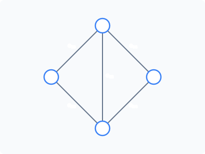
Delete row 4 and column 4:

$L_4 = \begin{pmatrix} 3 & -1 & -1 \\ -1 & 3 & -1 \\ -1 & -1 & 2 \end{pmatrix}$

$\det(L_4) = 3(3\cdot2 - (-1)(-1)) - (-1)((-1)\cdot2 - (-1)(-1)) + (-1)((-1)(-1) - 3(-1)) = 15 - 3 - 4 = 8$

So the theorem predicts 8 spanning trees. That’s checkable independently: $K_4$ has 16 spanning trees total (Cayley’s formula), and by the symmetry of $K_4$ every one of its 6 edges appears in the same number of them. Each tree has 3 edges, so summing edge-appearances across all 16 trees gives $16 \times 3 = 48$, spread evenly over 6 edges, meaning each edge appears in $48/6 = 8$ trees. The trees that survive removing edge $34$ are exactly the ones that never used it: $16 - 8 = 8$. Both routes agree.

Why this beats enumeration

The determinant of an $n \times n$ matrix can be computed via Gaussian elimination in $O(n^3)$ time. Directly enumerating spanning trees, by contrast, is exponential in the worst case, the number of trees itself grows exponentially (a dense graph on 20 vertices can easily have trillions of spanning trees), so no algorithm that lists them one at a time can keep up. The Matrix-Tree theorem sidesteps the listing entirely: it gets the count out of a computation whose cost barely notices how large that count is.

Electrical networks: where the same matrix reappears

Kirchhoff didn’t arrive at this theorem through graph theory. He was analysing resistor networks, and the Laplacian shows up there too, under a different name, as the conductance matrix. If every edge is a 1-ohm resistor, injecting current at one node and extracting it at another produces node voltages governed by exactly the linear system $Lv = i_{\text{ext}}$ (with one node grounded as a reference, since $L$ itself is singular).

Solving that system with Cramer’s rule brings back the same cofactors that count spanning trees, and the result is a second classical formula, also due to Kirchhoff: the effective resistance between nodes $a$ and $b$ is

$R_{\text{eff}}(a,b) = \frac{T_{a,b}(G)}{\tau(G)}$

where $\tau(G)$ is the total spanning tree count as before, and $T_{a,b}(G)$ counts spanning 2-forests that separate $a$ and $b$: subsets of $n-2$ edges that form exactly two trees covering all $n$ vertices between them, with $a$ in one and $b$ in the other. The derivation follows the same Cauchy-Binet pattern as the main proof, just applied to the numerator and denominator of Cramer’s rule instead of to a single determinant, so it won’t be repeated in full here, but the machinery is identical.

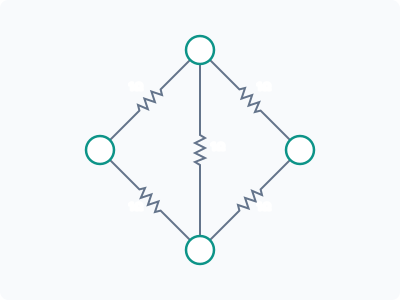
Checking this against the diamond graph: we already know $\tau(G) = 8$. For $T_{3,4}(G)$, count the 2-edge forests that put vertices 3 and 4 in different components. There are $\binom{5}{2} = 10$ ways to choose 2 edges from the graph’s 5 edges, and since no two edges share both endpoints, every pair is automatically a forest. Going through all 10 pairs, 8 of them separate vertex 3 from vertex 4, and only the two pairs that route both edges through a single shared vertex adjacent to both (${13,14}$ and ${23,24}$) keep 3 and 4 in the same component. So $T_{3,4}(G) = 8$, giving

$R_{\text{eff}}(3,4) = \frac{8}{8} = 1 \text{ ohm}$

Solving the circuit directly, by writing out Kirchhoff’s current law at each node with 1 amp injected at vertex 3 and extracted at vertex 4, and grounding vertex 2, confirms the same answer: $V_3 - V_4 = 1$. The graph-counting formula and the direct circuit solution land on the same number, because they’re computing the same determinant from two different starting points.

The broader pattern

What makes this theorem satisfying isn’t just that the formula works, it’s that a single matrix, built from purely local information (which vertices are adjacent to which), encodes a global combinatorial count that has no obvious reason to be computable so cheaply. The same object, reduced the same way, also happens to answer a completely different physical question about current flow. That’s not a coincidence so much as a reflection of the fact that spanning trees and current flow are, underneath, the same linear algebra: both are asking how many independent ways there are to route a single unit of flow through a graph without creating a cycle.