The Graph Fourier Transform: From Sinusoids to Eigenvectors

The ordinary Fourier transform decomposes a signal into frequencies, and “frequency” makes intuitive sense when your signal lives on a line or a circle: it’s how fast a sine wave oscillates as you walk along that line. But plenty of data doesn’t live on a line. Sensor readings sit on the nodes of a sensor network. Traffic measurements sit on a road graph. A signal on a social network is one number per user, connected in whatever irregular way friendships happen to connect them. There’s no natural direction to walk in, so “how fast does this oscillate” stops meaning anything obvious.

And yet there’s a well defined way to talk about frequency on a graph, and it turns out to be exactly the machinery from the last article. The eigenvectors of the graph Laplacian play the same role that sine and cosine waves play for ordinary Fourier analysis, and the connection isn’t just an analogy, it’s the same underlying idea (decomposing a signal into the eigenbasis of a particular operator) applied to two different domains, one continuous and one discrete.

Part 1: what frequency actually is

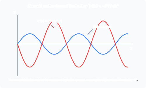
Start with a periodic function $f$ on the circle, meaning $f(x) = f(x + 2\pi)$. The building blocks of its Fourier series are the complex exponentials $e^{ikx}$ for integer $k$. Differentiate one twice:

$\frac{d}{dx} e^{ikx} = ik \, e^{ikx}, \qquad \frac{d^2}{dx^2} e^{ikx} = (ik)^2 e^{ikx} = -k^2 e^{ikx}$

So $e^{ikx}$ is an eigenfunction of the second-derivative operator, with eigenvalue $-k^2$. Flip the sign and write $\mathcal{L} = -\dfrac{d^2}{dx^2}$ (calling it $\mathcal{L}$ deliberately, this is the continuous Laplacian), and

$\mathcal{L} \, e^{ikx} = k^2 \, e^{ikx}$

This is the entire content of the claim “sinusoids are the natural frequency basis”: they are, quite literally, the eigenfunctions of the Laplacian operator, and the eigenvalue $k^2$ is what we’ve been informally calling the frequency squared. The Fourier transform isn’t a separate piece of machinery bolted onto calculus, it’s an eigendecomposition.

Why the Laplacian specifically, and not some other operator? Because $\mathcal{L}$ measures local roughness. For a function $f$, the Dirichlet energy $\int |f'(x)|^2 \, dx$ quantifies how much $f$ oscillates: a flat function has zero Dirichlet energy, a wildly oscillating one has a large one. Expand $f$ in its Fourier series, $f(x) = \sum_k c_k e^{ikx}$, differentiate term by term, and use the orthogonality relation $\int_0^{2\pi} e^{ikx} e^{-ijx}\,dx = 2\pi \, \delta_{kj}$:

$\int_0^{2\pi} |f'(x)|^2\, dx = \sum_k \sum_j c_k \overline{c_j} (ik)(\overline{ij}) \int_0^{2\pi} e^{i(k-j)x}\,dx = 2\pi \sum_k k^2 |c_k|^2$

The cross terms vanish by orthogonality, and what survives is a direct correspondence: the roughness of $f$ is exactly a weighted sum of its Fourier coefficients, weighted by $k^2$, the eigenvalue attached to each mode. High-frequency modes carry more of the roughness, low-frequency modes carry less, and the constant mode $k=0$ carries none at all. Frequency, roughness, and eigenvalue of the Laplacian are three names for the same quantity.

That last identity is the thread to pull on. It doesn’t actually use anything about the circle specifically, translation invariance, periodicity, none of it enters the argument. All it needs is an operator that measures roughness and a basis that diagonalises it. A graph has no translations to speak of, but it absolutely has a notion of roughness, and it has an operator to match.

Part 2: the graph version

A graph signal is just a function $f : V \to \mathbb{R}$, one real number per vertex. The graph Laplacian from before, $L = D - A$, is the discrete stand-in for $\mathcal{L}$, and the parallel to Dirichlet energy is immediate. For any signal $f$,

$f^\top L f = \sum_{(i,j) \in E} (f_i - f_j)^2$

This is a direct calculation: $f^\top L f = f^\top D f - f^\top A f = \sum_i d_i f_i^2 - \sum_{(i,j)\in E} 2 f_i f_j$, and regrouping the sum edge by edge turns this into $\sum_{(i,j)\in E}(f_i-f_j)^2$. It’s non-negative for every $f$ (it’s a sum of squares), which is why $L$ is positive semidefinite, and it’s the exact discrete analogue of $\int |f'|^2\,dx$: instead of measuring how much $f$ changes over an infinitesimal step along a line, it measures how much $f$ changes across each edge of the graph.

Because $L$ is real and symmetric, the spectral theorem guarantees an orthonormal basis of eigenvectors $u_1, \dots, u_n$ with real eigenvalues $0 = \lambda_1 \le \lambda_2 \le \cdots \le \lambda_n$. Collect the eigenvectors as columns of an orthogonal matrix $U$. The Graph Fourier Transform of a signal $f$ is defined as

$\hat{f} = U^\top f, \qquad f = U \hat{f} = \sum_k \hat{f}_k \, u_k$

exactly mirroring the Fourier series, a signal written as a weighted sum of fixed basis modes. And because $f = U\hat{f}$ diagonalises the quadratic form,

$f^\top L f = (U\hat f)^\top L (U\hat f) = \hat f^\top (U^\top L U) \hat f = \hat f^\top \Lambda \hat f = \sum_k \lambda_k \, \hat{f}_k^2$

which is the discrete Parseval identity: total roughness equals the sum of squared Fourier coefficients weighted by eigenvalue, the same relationship derived above for the circle, except the finite-dimensional version falls out in one line of linear algebra instead of an integration by parts. The eigenvalue $\lambda_k$ is the graph’s notion of $k^2$: small $\lambda_k$ means the eigenvector $u_k$ is nearly constant across every edge (low frequency, smooth), large $\lambda_k$ means $u_k$ flips sign or swings wildly between neighbours (high frequency, rough). The smallest eigenvalue is always $\lambda_1 = 0$, achieved by the constant vector (every row of $L$ sums to zero), playing the role of the $k=0$ DC component in the continuous case.

Part 3: an exact case where the analogy is not an analogy

For most graphs the eigenvectors of $L$ have no closed form, you compute them numerically and that’s that. But for one important family, the cycle graph $C_n$ (vertices $0, \dots, n-1$ arranged in a ring, each connected to its two neighbours), the eigenvectors work out exactly, and they turn out to be the classical discrete Fourier basis itself.

The Laplacian of $C_n$ has a special structure: every row is the previous row shifted over by one, because every vertex looks identical to every other vertex up to relabelling. A matrix with this property is called circulant: $C_{jk} = c_{(k-j)\bmod n}$ for some fixed sequence $c_0, \dots, c_{n-1}$ (the “first row”).

Claim. Every circulant matrix has eigenvectors $v_m = (1, \omega^m, \omega^{2m}, \dots, \omega^{(n-1)m})$, for $m = 0, \dots, n-1$, where $\omega = e^{2\pi i/n}$, with eigenvalue $\mu_m = \sum_{l=0}^{n-1} c_l \, \omega^{ml}$.

Proof. Compute the $j$-th entry of $Cv_m$ directly:

$(Cv_m)_j = \sum_{k=0}^{n-1} C_{jk} (v_m)_k = \sum_{k=0}^{n-1} c_{(k-j)\bmod n} \, \omega^{mk}$

Substitute $l = (k-j) \bmod n$, so $k \equiv j + l \pmod n$ and $\omega^{mk} = \omega^{m(j+l)} = \omega^{mj}\omega^{ml}$ (this holds even across the wraparound because $\omega^n = 1$). As $k$ ranges over $0, \dots, n-1$, $l$ ranges over the same set, so

$(Cv_m)_j = \sum_{l=0}^{n-1} c_l \, \omega^{mj}\omega^{ml} = \omega^{mj} \sum_{l=0}^{n-1} c_l \,\omega^{ml} = \mu_m \, (v_m)_j$

for every $j$, so $Cv_m = \mu_m v_m$. $\blacksquare$

This proof used nothing about $C_n$ specifically, it’s a general fact about any circulant matrix. Now apply it. The Laplacian of $C_n$ has first row $c_0 = 2$ (the degree), $c_1 = -1$ (the clockwise neighbour), $c_{n-1} = -1$ (the counterclockwise neighbour), and zero everywhere else. Plugging into the formula for $\mu_m$:

$\mu_m = 2 - \omega^m - \omega^{-m} = 2 - 2\cos\!\left(\frac{2\pi m}{n}\right) = 4\sin^2\!\left(\frac{\pi m}{n}\right)$

using $\omega^m + \omega^{-m} = 2\cos(2\pi m/n)$ and the half-angle identity $1 - \cos\theta = 2\sin^2(\theta/2)$. So the eigenvalues of the cycle Laplacian are $\lambda_m = 4\sin^2(\pi m/n)$, and the eigenvectors are $v_m(j) = \omega^{mj} = e^{2\pi i mj/n}$: the exact complex exponential basis of the classical discrete Fourier transform, on the nose. On a cycle, the Graph Fourier Transform is the DFT, not an analogue of it. (Pairing up $m$ and $n-m$, which share the same eigenvalue since $\sin^2$ is symmetric about $\pi/2$, and taking real and imaginary parts recovers real sine and cosine eigenvectors, exactly as combining $e^{ikx}$ and $e^{-ikx}$ recovers real sinusoids in the continuous case.)

As a check, take $n=4$: $\lambda_m = 4\sin^2(\pi m/4)$ gives $\lambda_0 = 0$, $\lambda_1 = 4 \cdot \tfrac12 = 2$, $\lambda_2 = 4 \cdot 1 = 4$, $\lambda_3 = 4 \cdot \tfrac12 = 2$. Four vertices, eigenvalues $\{0, 2, 4, 2\}$, one zero mode, two mirror-image frequency-1 modes at $\lambda = 2$, and one fastest-oscillating mode at $\lambda = 4$ where adjacent vertices alternate sign. That last one is the graph equivalent of the highest frequency a 4-sample signal can represent, the discrete analogue of the Nyquist limit.

Part 4: a worked example on an irregular graph

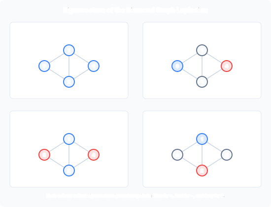
Cycles are convenient because of the symmetry, but the whole point of the graph Fourier transform is that it works on graphs with no symmetry at all. The diamond graph from the spanning tree article (vertices $1,2,3,4$, edges $12,13,14,23,24$) has less symmetry than a cycle but still enough to get a clean answer by hand, using its automorphisms directly: swapping vertices $1 \leftrightarrow 2$ leaves the graph unchanged, and so does swapping $3 \leftrightarrow 4$, independently. Any eigenvector must be symmetric or antisymmetric under each of those swaps, which splits the $4\times 4$ eigenvalue problem into small independent pieces.

Solving each piece (the algebra is routine, so only the results are shown) gives eigenvalues $\{0, 2, 4, 4\}$ with orthogonal eigenvectors

$u_1 = \tfrac{1}{2}(1,1,1,1), \quad u_2 = \tfrac{1}{\sqrt2}(0,0,1,-1), \quad u_3 = \tfrac{1}{2}(1,1,-1,-1), \quad u_4 = \tfrac{1}{\sqrt2}(1,-1,0,0)$

$u_1$ is the constant mode, zero frequency, as always. $u_2$ oscillates only between the two low-degree vertices $3$ and $4$. $u_3$ and $u_4$ both sit at the top eigenvalue $\lambda = 4$, the fastest disagreement the graph can support, one splitting the high-degree pair from the low-degree pair, the other splitting the two high-degree vertices from each other.

Take a signal, say a temperature reading at each vertex: $f = (10, 8, 3, 1)$. Its graph Fourier transform is $\hat f = U^\top f$:

$\hat f_1 = u_1 \cdot f = \tfrac12(22) = 11, \quad \hat f_2 = u_2\cdot f = \tfrac{1}{\sqrt2}(2) = \sqrt2$ $\hat f_3 = u_3\cdot f = \tfrac12(14) = 7, \quad \hat f_4 = u_4\cdot f = \tfrac{1}{\sqrt2}(2) = \sqrt2$

The dominant coefficient is $\hat f_1 = 11$, the mean level of the signal, exactly as the DC term dominates a smooth continuous signal. The two $\lambda=4$ coefficients are comparatively small, meaning the signal doesn’t disagree much between the high-degree pair or between the low-degree pair, most of the actual variation is captured by the low and mid frequency terms.

Low-pass filtering. Attenuating the high-frequency coefficients and reconstructing is exactly what a graph low-pass filter does. Zeroing out the $\lambda=4$ terms entirely and inverting:

$f_{\text{filtered}} = \hat f_1 u_1 + \hat f_2 u_2 = 11\cdot\tfrac12(1,1,1,1) + \sqrt2\cdot\tfrac{1}{\sqrt2}(0,0,1,-1) = (5.5,\, 5.5,\, 6.5,\, 4.5)$

The sharp local disagreements are smoothed out while the overall shape of the signal (high near vertices 1,2, tapering toward 3,4) survives. This is the same operation as blurring an image, just performed on an arbitrary graph instead of a pixel grid.

Part 5: filtering is diffusion

The low-pass filter above was done by hand, picking which coefficients to zero out. There’s a more principled way to choose the attenuation, and it comes from the same operator playing a third role: governing diffusion.

The continuous heat equation $\partial u/\partial t = -\mathcal{L}u$ describes how heat spreads out over time. Solved in the Fourier basis, each mode decays independently: $u(x,t) = \sum_k c_k(0) \, e^{-k^2 t} \, e^{ikx}$, high-frequency components (large $k^2$) die out fast, low-frequency components persist. That’s why heat diffusion looks like blurring: it’s a low-pass filter that runs continuously in time rather than being applied in one discrete step.

The graph version is identical in structure. The graph heat equation $\dot u = -Lu$ has solution $u(t) = e^{-tL} u(0)$, and expanding in the eigenbasis,

$u(t) = \sum_k e^{-t\lambda_k} \, \hat u_k(0) \, u_k$

Each graph-frequency component decays at a rate set by its own eigenvalue, exactly mirroring the continuous case term for term. Letting this run for a short time $t$ is a low-pass filter, a soft, continuously tunable version of the hard cutoff used in the worked example above: instead of zeroing high-frequency coefficients outright, they’re scaled down by $e^{-t\lambda_k}$, with larger $t$ suppressing more of the spectrum. Graph filtering and graph diffusion aren’t two separate applications sitting next to each other, they’re the same computation, viewed either as a signal-processing operation or as a physical process running on the graph.

Where the analogy breaks

The comparison holds up remarkably well, but it isn’t perfect. The circle has translation symmetry: shifting a function and then Fourier transforming gives the same result as transforming and then shifting, and this is exactly why the same $e^{ikx}$ basis works everywhere on the circle regardless of where you start counting. Most graphs have no such symmetry (the diamond graph example only had it because of its particular automorphisms), so the graph Fourier basis is tied to the specific graph you built it from. There’s no universal graph-frequency basis the way there’s a universal continuous one, every graph gets its own, computed from its own Laplacian. The idea generalises cleanly; the specific basis functions do not.