JK and T Flip-Flops
The JK Flip-Flop
The RS latch has a forbidden state when R = S = 1. The JK flip-flop eliminates this restriction by redefining the J = K = 1 condition to produce a useful behaviour: toggle. When both inputs are asserted, the output toggles (Q’ = Q̄).
The JK flip-flop is named after Jack Kilby (inventor of the integrated circuit), though the naming is incidental to our purposes. Its behaviour is:
| J | K | Q’ | Q̄’ | Comment |
|---|---|---|---|---|
| 0 | 0 | Q | Q̄ | Hold |
| 0 | 1 | 0 | 1 | Reset |
| 1 | 0 | 1 | 0 | Set |
| 1 | 1 | Q̄ | Q | Toggle |
Where Q’ is the next state after the clock edge and Q is the current state before the edge.
Internal Structure (Conceptual)
The JK flip-flop’s internal structure uses a master-slave configuration with feedback from the outputs to the input gating. The J and K inputs are combined with Q and Q̄ to ensure the toggle behaviour works correctly:
- The gating logic prevents J = K = 1 from causing a race condition. The feedback ensures that during the toggle, the master and slave never both try to set simultaneously.
- Because of the master-slave structure, there is a constraint: J and K must remain stable while the clock is high (the “1s catching” problem). Input changes during CLK = 1 can cause unintended behaviour. Modern JK flip-flops use edge-triggered designs to eliminate this issue.
State Diagram
The JK flip-flop has two states (Q = 0 and Q = 1) with the following transitions labelled J,K:
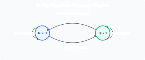
Arcs labelled:
- From Q = 0 to Q = 0: J = 0, K = X (hold) or J = X, K = 0 (hold)
- From Q = 0 to Q = 1: J = 1, K = X (set) or J = 1, K = 1 (toggle)
- From Q = 1 to Q = 0: J = X, K = 1 (reset) or J = 1, K = 1 (toggle)
- From Q = 1 to Q = 1: J = X, K = 0 (hold) or J = 0, K = X (hold)
The key difference from the SR flip-flop: J = K = 1 is allowed and produces a toggle (Q’ = Q̄). This eliminates the forbidden state problem of the SR flip-flop.
The T (Toggle) Flip-Flop
The T flip-flop is a JK flip-flop with J and K permanently tied together and renamed as the T input:
| T | Q’ | Q̄’ | Comment |
|---|---|---|---|
| 0 | Q | Q̄ | Hold |
| 1 | Q̄ | Q | Toggle |
When T = 0, the FF holds its state (J = K = 0 → hold). When T = 1, the FF toggles on each clock edge (J = K = 1 → toggle).
The T flip-flop is the natural building block for counters: by connecting T = 1 permanently, the FF toggles on every clock edge, halving the frequency at each stage. The ripple counter and synchronous counter designs in /modules/digital-electronics/07-flip-flop-applications-and-timing/01-ripple-counters/ use this principle.
Characteristic Equations
The characteristic equation gives the next state Q’ as a function of the current state Q and the inputs. These are the defining equations for each FF type:
-
D flip-flop:
-
JK flip-flop:
Verify: J = 0, K = 0 → Q’ = 0 + 1·Q = Q (hold). J = 0, K = 1 → Q’ = 0 + 0·Q = 0 (reset). J = 1, K = 0 → Q’ = 1·Q̄ + 1·Q = Q̄ + Q = 1 (set). J = 1, K = 1 → Q’ = 1·Q̄ + 0·Q = Q̄ (toggle).
-
T flip-flop:
When T = 0: Q’ = Q (hold). When T = 1: Q’ = Q̄ (toggle). This is simply an XOR of T with Q.
Excitation Tables
For FSM design, we need to know what inputs to apply to achieve a desired state transition. This is the excitation table, which answers: “Given current state Q and desired next state Q’, what values must the FF inputs take?”
D flip-flop excitation table (trivial: D must equal the desired Q’):
| Q | Q’ | D |
|---|---|---|
| 0 | 0 | 0 |
| 0 | 1 | 1 |
| 1 | 0 | 0 |
| 1 | 1 | 1 |
Since D = Q’, the excitation is independent of Q. For D-FFs, the FF input column in a state transition table is always identical to the next-state column.
JK flip-flop excitation table:
| Q | Q’ | J | K |
|---|---|---|---|
| 0 | 0 | 0 | X |
| 0 | 1 | 1 | X |
| 1 | 0 | X | 1 |
| 1 | 1 | X | 0 |
X means “don’t care”: either 0 or 1 works equally well. For the transition 0 → 0, either hold (J = 0, K = 0) or reset (J = 0, K = 1, which holds a 0 at 0) works. For 0 → 1, either set (J = 1, K = 0) or toggle (J = 1, K = 1, which toggles 0 to 1) works. The don’t-cares give flexibility in logic minimisation.
T flip-flop excitation table:
| Q | Q’ | T |
|---|---|---|
| 0 | 0 | 0 |
| 0 | 1 | 1 |
| 1 | 0 | 1 |
| 1 | 1 | 0 |
T = Q ⊕ Q’: the T input is simply the XOR of the current and next states.
Why JK and T FFs Matter
Historically, JK flip-flops were widely used in discrete logic designs (74-series chips) because the toggle feature and the don’t-care inputs simplified the next-state logic. T flip-flops are the natural choice for counters: connect T = 1 for a toggle-on-every-clock, or derive T from a simple AND of lower-order counter bits for a synchronous counter.
In modern designs (FPGAs, ASICs), D flip-flops dominate because they are simpler to implement in silicon and the synthesis tools handle the next-state logic automatically. However, the JK and T FF concepts remain important for understanding counter design and for Tripos questions that require the excitation table approach. The Tripos question in /modules/digital-electronics/08-synchronous-state-machines/05-fsm-tripos-example/ uses D-FFs with the excitation table method.