Metastability

What Is Metastability?

A flip-flop is a bistable device: it has two stable states (Q = 0 and Q = 1). When the setup or hold time is violated, the internal feedback loop may not cleanly resolve to either state. Instead, the output hovers at an intermediate voltage: neither a valid logic 0 nor a valid logic 1. This condition is called metastability.

The ball-on-hill analogy: two valleys represent the stable states (0 and 1). The summit is the metastable state. If the ball is placed exactly on the summit (perfect balance), it stays there. In reality, thermal noise and circuit imbalances cause the ball to eventually roll into one valley. The time this takes depends on how close to perfectly balanced the initial condition was.

The critical point: the resolution time is unbounded. In theory, the FF could remain metastable indefinitely. In practice, the probability of remaining metastable for time t decreases exponentially with t.

When Does Metastability Occur?

Metastability is triggered when the D input changes within the setup-hold window around the clock edge. This is unavoidable when:

• An asynchronous signal (e.g., a button press, an external sensor) is sampled by a clocked system.
• Data arrives from a different clock domain (different frequency or phase).
• Clock skew or excessive combinational delay causes a violation.

In synchronous systems where all paths meet timing, metastability does not occur within the core logic. It becomes an issue at boundaries: inputs from the outside world, or crossing between clock domains.

The Probability Model

The probability that the resolution time t_res exceeds some time t is given by:

$P(t_{res} > t) = \frac{T_0}{T_c} e^{-t/\tau}$

Where:

• T_c is the clock period
• T₀ and τ (tau) are device-specific parameters
  • τ is the regeneration time constant: inversely proportional to the gain-bandwidth product of the FF’s internal feedback loop. Smaller τ means faster resolution. Typical values are tens of picoseconds.
  • T₀ / T_c is approximately the probability that the input changes during the vulnerable setup-hold window in a given clock cycle.

The probability has two factors:

1. T₀ / T_c: the chance of hitting the bad timing window (proportional to the width of the window divided by the clock period).
2. e^-t/τ: given that metastability occurs, the probability that it persists longer than t. This decreases exponentially with waiting time.

Synchronisers: Reducing the Probability

A synchroniser is a chain of two (or more) FFs in series, sharing the same clock, used to safely bring an asynchronous signal into the clocked domain:

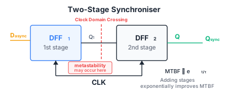
FF0 samples the asynchronous D_in. If a timing violation occurs, FF0’s output Q might go metastable. However, FF0 has an entire clock period to resolve before FF1 samples Q on the next clock edge. The resolution time available is t_res = T_c - t_su.

If Q resolves within that time, FF1 sees a clean 0 or 1 and produces a glitch-free output. The probability that FF1 itself goes metastable (i.e., the synchroniser fails) is:

$P_{fail} = \frac{T_0}{T_c} e^{-(T_c - t_{su})/\tau}$

Mean Time Between Failures (MTBF)

For a system where the asynchronous input changes N times per second, the failure rate is N · P_fail (failures per second). The Mean Time Between Failures is the reciprocal:

$MTBF = \frac{1}{N \cdot P_{fail}} = \frac{T_c}{N \cdot T_0} e^{(T_c - t_{su})/\tau}$

This is the key metric for synchroniser reliability.

Worked Example: MTBF Calculation

FFs in a synchroniser have: τ = 200 ps, T₀ = 150 ps, t_su = 500 ps. The asynchronous input changes N = 0.2 times per second on average. What clock period T_c gives MTBF ≥ 1 year?

1 year ≈ π × 10⁷ ≈ 31.5 × 10⁶ seconds.

$31.5 \times 10^6 = \frac{T_c}{0.2 \times 150 \times 10^{-12}} e^{(T_c - 500 \times 10^{-12}) / (200 \times 10^{-12})}$

This transcendental equation has no closed-form solution. Solving by trial and error:

Try T_c = 3 ns: exponent = (3000 - 500)/200 = 12.5; e¹²·⁵ ≈ 2.68 × 10⁵. Coefficient = 3×10⁻⁹ / (0.03×10⁻⁹) = 100. MTBF = 100 × 2.68×10⁵ = 2.68×10⁷ s ≈ 0.85 years (too low).

Try T_c = 3.04 ns: exponent ≈ 12.7; e¹²·⁷ ≈ 3.28×10⁵. MTBF ≈ 101.3 × 3.28×10⁵ ≈ 3.32×10⁷ s ≈ 1.05 years. This meets the requirement.

What if we tried T_c = 2 ns? exponent = (2000-500)/200 = 7.5; e⁷·⁵ ≈ 1808. MTBF ≈ 66.7 × 1808 ≈ 1.21×10⁵ s ≈ 1.4 days! The exponential sensitivity means a small reduction in resolution time produces a catastrophic drop in reliability.

The Exponential Magic

The exponential in the MTBF formula is what makes synchronisers work. With conservative timing (sufficient T_c), MTBF can be astronomical: billions of years, far exceeding the age of the universe. This sounds absurd but is a standard result in the literature.

The danger is if the designer “starves” the synchroniser: reducing the clock period to boost performance without checking the MTBF. Going from T_c = 3.04 ns to T_c = 2 ns reduced MTBF from 1 year to 1.4 days in the example above. This is why synchroniser timing must be verified independently of the main design.

Cascaded Synchronisers (K Extra FFs)

For even higher reliability, additional FFs can be cascaded. If each additional FF independently has failure probability P_fail, then K extra FFs give:

$P_{fail\_K} = (P_{fail})^K$

$MTBF_K = \frac{1}{N \cdot (P_{fail})^K}$

This improves reliability dramatically provided P_fail ≪ 1. If P_fail = 10⁻⁶, then with K = 2, P_{fail_K} = 10⁻¹². Two extra FFs (three total) is the conventional design: one to resolve, one to capture cleanly, and optionally a third to guard against extreme conditions.

Design Rules for Synchronisers

• Never feed an asynchronous signal directly into the core logic. Always pass it through a synchroniser first.
• Do not use the output of the first FF of a synchroniser for anything except feeding the second FF. The first output may be metastable for most of the clock period.
• Keep the synchroniser FFs physically close together (minimise wire delay between them).
• Verify synchroniser MTBF at the target clock frequency. It must exceed the expected product lifetime.
• Be aware that different bits of a multi-bit asynchronous bus must be synchronised independently; simple synchronisers do not guarantee the bits are captured in the same cycle. For multi-bit transfers, use a handshake protocol or an asynchronous FIFO.